New original cover art included with this eBook is granted to the public domain.
BY
CHARLES N. PICKWORTH
WHITWORTH SCHOLAR; EDITOR OF “THE MECHANICAL WORLD”; AUTHOR OF “LOGARITHMS FOR BEGINNERS”; “THE INDICATOR: ITS CONSTRUCTION AND APPLICATION”; “THE INDICATOR DIAGRAM: ITS ANALYSIS AND CALCULATION,” ETC.
SEVENTEENTH EDITION
Manchester:
Emmott and Co., Limited,
65 King Street;
New York:
D. Van Nostrand Co.,
8 Warren Street.
London:
Emmott and Co., Limited,
20 Bedford Street, W.C.
and
Pitman and Sons, Limited,
Parker St., Kingsway, W.C. 2.
[Three Shillings and Sixpence net]
All rights reserved.
PREFACE TO THE FIFTEENTH EDITION. — PREFACE TO THE SEVENTEENTH EDITION.
Several new slide rules for special calculations are described in
this edition, and the contents further extended to include a
section dealing with screw-cutting gear calculations by the slide rule—an
application of the instrument to which attention has been given
recently.
Mention should be made of the fact that some of the special slide
rules described in previous editions are no longer obtainable. As,
however, the descriptive notes may be of service to those possessing
the instruments, and are, in some measure, of general interest, they
have been allowed to remain in the present issue.
The author tenders his thanks to the many who have evinced their
appreciation of his efforts to popularise the subject; also for the many
kind hints and suggestions which he has received from time to time,
and with a continuance of which he trusts to be favoured in the
future.
C. N. P.
Withington, Manchester, November 1917.
The sustained demand for this very successful work having
resulted in the early call for a new edition, the opportunity
has been taken to introduce descriptions of new slide rules and to
effect some slight revisions.
The slide rule may be defined as an instrument for mechanically
effecting calculations by logarithms. Those familiar
with logarithms and their use will recognise that the slide rule
provides what is in effect a concisely arranged table of logarithms,
together with a simple and convenient means for adding and
subtracting any selected values. Those, however, who have no
acquaintance with logarithms will find that only an elementary
knowledge of the subject is necessary to enable them to make full
use of the slide rule. It is true that for simple slide-rule operations,
as multiplication and division, a knowledge of logarithms is
unnecessary; indeed, many who have no conscious understanding
of logarithms make good use of the instrument. But this involves
a blind reliance upon rules without an appreciation of their origin
or limitations, and this, in turn, engenders a want of confidence in
the results of any but the simplest operations, and prevents the
fullest use being made of the instrument. For this reason a brief,
but probably sufficient résumé of the principles of logarithmic
calculation will be given. Those desiring a more detailed explanation
are referred to the writer’s “Logarithms for Beginners.”
The slide rule enables various arithmetical, algebraical and
trigonometrical processes to be performed with ease and rapidity,
and with sufficient accuracy for most practical purposes. A grasp
of the simple fundamental principles which underlie its operation,
together with a little patient practice, are all that are necessary to
acquire facility in using the instrument, and few who have become
proficient in this system of calculating would willingly revert to
the laborious arithmetical processes.
THE MATHEMATICAL PRINCIPLE OF THE SLIDE RULE.
6
Logarithms may be defined as a series of numbers in arithmetical
progression, as 0, 1, 2, 3, 4, etc., which bear a definite relationship
to another series of numbers in geometrical progression, as 1, 2, 4,
8, 16, etc. A more precise definition is:—The logarithm of a
number to any base, is the index of the power to which the base
must be raised to equal the given number. In the logarithms in
general use, known as common logarithms, and with which we are
alone concerned, 10 is the base selected. The general definition
may therefore be stated in the following modified form:—The
common logarithm of a number is the index of the power to which
10 must be raised to equal the given number. Applying this rule
to a simple case, as 100 = 102, we see that the base 10 must be
squared (i.e., raised to the 2nd power) in order to equal 100, the
number selected. Therefore, as 2 is the index of the power to
which 10 must be raised to equal 100, it follows from our definition
that 2 is the common logarithm of 100. Similarly the common
logarithm of 1000 will be 3, while proceeding in the opposite
direction the common log. of 10 must equal 1. Tabulating these
results and extending, we have:—
Numbers
10,000
1000
100
10
1
Logarithms
4
3
2
1
0
It will now be evident that for numbers
between
1
and
10
the logs. will be between
0
and
1
„
10
„
100
„ „
1
„
2
„
100
„
1000
„ „
2
„
3
„
1000
„
10,000
„ „
3
„
4
In other words, the logarithms of numbers between 1 and 10 will
be wholly fractional (i.e., decimal); the logs. of numbers between
10 and 100 will be 1 followed by a decimal quantity; the logs. of
numbers between 100 and 1000 will be 2 followed by a decimal
quantity, and so on. These decimal quantities for numbers from
1 to 10 (which are the logarithms of this particular series) are
as follows:—
Numbers
1
2
3
4
5
6
7
8
9
10
Logarithms
0
0·301
0·477
0·602
0·699
0·778
0·845
0·903
0·954
1·000
7Combining the two tables, we can complete the logarithms. Thus
for 3 multiplied successively by 10, we have:—
Numbers
3
30
300
3000
30,000
etc.
Logarithms
0·477
1·477
2·477
3·477
4·477
We see from this that for numbers having the same significant
figure (or figures), 3 in this case, the decimal part or mantissa of
the logarithm is the same, but that the integral part or characteristic
is always one less than the number of figures before the decimal
point.
For numbers less than 1 the same plan is followed. Thus
extending our first table downwards, we have:—
Numbers
1
0·1
0·01
0·001
0·0001
etc.
Logarithms
0
−1
−2
−3
−4
so that for 3 divided successively by 10, we have:—
Numbers
3
0·3
0·03
0·003
0·0003
etc.
Logarithms
0·477
̅1·477
̅2·477
̅3·477
̅4·477
Here again we see that with the same significant figures in the
numbers, the mantissa of the logarithm has always the same
(positive) value, but the characteristic is one more than the number
of 0’s immediately following the decimal point, and is negative, as
indicated by the minus sign written over it. Only the decimal
parts of the logarithms of numbers between 1 and 10 are given
in the usual tables, for, as shown above, the logarithms of all tenfold
multiples or submultiples of a number can be obtained at
once by modifying the characteristic in accordance with the rules
given.
An examination of the two rows of figures giving the logarithms
of numbers from 1 to 10 will reveal some striking peculiarities,
and at the same time serve to illustrate the principle of logarithmic
calculation. First, it will be noticed that the addition of any two
of the logarithms gives the logarithm of the product of these two
numbers. Thus, the addition of log. 2 and log. 4 = 0·301 + 0·602
= 0·903, and this is seen to be the logarithm of 8, that is, of 2 × 4.
Conversely, the difference of the logarithms of two numbers gives
the logarithm of the quotient resulting from the division of these
two numbers. Thus, log. 8 − log. 2 = 0·903 − 0·301 = 0·602, which is
the log. of 4, or of 8 ÷ 2.
8One other important point is to be noted. If the logarithm of
any number is multiplied by 2, 3, or any other quantity, whole or
fractional, the result is the logarithm of the original number,
raised to the 2nd, 3rd, or other power respectively. Thus, multiplying
the log. of 3 by 2, we obtain 0·477 × 2 = 0·954, and this is
seen to be the log. of 9, that is, of 3 raised to the 2nd power, or 3
squared. Again, log. 2 multiplied by 3 = 0·903—that is, the log. of
8, or of 2 raised to the 3rd power, or 2 cubed. Conversely, dividing
the logarithm of any original number by any number n, we obtain
the logarithm of the nth root of the original number. Thus, log.
8 ÷ 3 = 0·903 ÷ 3 = 0·301, and is therefore equal to log. 2 or to the
log. of the cube root of 8.
Only simple logs. have been taken in these examples, but the
student will understand that the same reasoning applies, whatever
the number. Thus for 203 we prefix the characteristic (1 in this
case) to log. 2, giving 1·301. Multiplying by 3, we have 3·903 as
the resulting logarithm, and as its characteristic is 3, we know
that it corresponds to the number 8000. Hence 203 = 8000.
In this brief explanation is included all that need now be said
with regard to the properties of logarithms. The main facts to
be borne clearly in mind are:—(1.) That to find the product of
two numbers, the logarithms of the numbers are to be added
together, the result being the logarithm of the product required,
the value of which can then be determined. (2.) That in finding
the quotient resulting from the division of one number by another,
the difference of the logarithms of the numbers gives the logarithm
of the quotient, from which the value of the latter can be ascertained.
(3.) That to find the result of raising a number to the nth
power, we multiply the logarithm of the number by n, thus obtaining
the logarithm, and hence the value, of the desired result. And
(4.) That to find the nth root of a number, we divide the logarithm
of the number by n, this giving the logarithm of the result, from
which its value may be determined.
NOTATION BY POWERS OF 10.
A convenient method of representing an arithmetical quantity is
to split it up into two factors, of which the first is the original
number, with the decimal point moved so as to immediately follow
the first significant figure, and the second, 10n where n is the
9number of places the decimal point has been moved, this index
being positive for numbers greater than 1, and negative for numbers
less than 1.[1] In this system, therefore, we regard 3,610,000 as
3·61 × 1,000,000, and write it as 3·61 × 106. Similarly 361 = 3·61 x 102;
0·0361 (=
3·61 100)
= 3·61 × 10−2; 0·0000361 = 3·61 × 10−5, etc. To restore
a number to its original form, we have only to move the
decimal point through the number of places indicated by the
index, moving to the right if the index is positive and to the
left (prefixing 0’s) if negative. This method, which should be
cultivated for ordinary arithmetical work, is substantially that
followed in calculating by the slide rule. Thus with the slide rule
the multiplication of 63,200 by 0·0035 virtually resolves itself into
6·32 × 104 × 3·5 × 10−3 or 6·32 × 3·5 × 104–3 = 22·12 x 101 = 221·2. It will
be seen later, however, that the result can be arrived at by a more
direct, if less systematic, method of working.
THE MECHANICAL PRINCIPLE OF THE SLIDE RULE.
Fig. 1.
The mechanical principle involved in the slide rule is of a very
simple character. In Fig. 1, A and B represent two rules divided
into 10 equal parts, the division lines being numbered consecutively
as shown. If the rule B is moved to the right until 0 on B is
opposite 3 on A, it is seen that any number on A is equal to the
coinciding number on B, plus 3. Thus opposite 4 on B is 7 on A.
The reason is obvious. By moving B to the right, we add to a
length 0·3, another length 0·4, the result read off on A being 7.
Evidently, the same result would have been obtained if a length
0·4 had been added, by means of a pair of dividers, to the length
0·3 on the scale A. By means of the slide B, however, the addition
is more readily effected, and, what is of much greater importance,
10the result of adding 3 to any one of the numbers within range, on
the lower scale, is immediately seen by reading the adjacent
number on A.
Of course, subtraction can be quite as readily performed.
Thus, to subtract 4 from 7, we require to deduct from 0·7 on the
A scale, a length 0·4 on B. We do this by placing 4 on B under
7 on A, when over 0 on B we find 3, on A. It is here evident that
the difference of any pair of coinciding numbers on the scales is
constantly equal to 3.
Fig. 2.
An important modification results if the slide-scale B is inverted
as in Fig. 2. In this case, to find the sum of 4 and 3 we
require to place the 4 of the A scale to 3 on the B scale, and the
result is read on A over 0 on B. Here it will be noted, the sum
of any pair of coinciding numbers on the scales is constant and
equal to 7. This case, therefore, resembles that of the immediately
preceding one, except that the sum, instead of the difference, of any
pair of coinciding numbers is constant.
To find the difference of two factors, the converse operation is
necessary. Thus, to subtract 4 from 7, 0 on B is placed opposite 7
on A, and over 4 on B is found 3 on A.
From these examples it will be seen that with the slide inverted
the methods of operation are the reverse of those used when the
slide is in its normal position.
It will be understood that although we have only considered
the primary divisions of the scales, the remarks apply equally to
any subdivisions into which the primary spaces of the scales might
be divided. Further, we note that the length of scale taken to
represent a unit is quite arbitrary.
THE PRIMITIVE SLIDE RULE.
The application of the foregoing principles to the slide rule can
be shown most conveniently by describing the construction of a
simple form of slide rule:—Take a strip of card about 11 in. long
and 2 in. wide; draw a line down the centre of its width, and
11mark off two points, 10 in. apart. Draw cross lines at these points
and figure them 1 and 10 on each side, as in Fig. 3. Next mark off
lengths of 3·01, 4·77, 6·02, 6·99, 7·78, 8·45, 9·03 and 9·54 inches,
from the line marked 1. Draw cross lines as before, and figure
these lines, 2, 3, 4, 5, 6, 7, 8 and 9. To fill in the intermediate
divisions of the scale, take the logs, of 1·1, 1·2, 1·3, etc. (from a
table), multiply each by 10, and thus obtain the distances from 1,
at which the several subdivisions are to be placed. Mark these
1·2, 1·3, 1·4, etc., and complete the scale, making the interpolated
division marks shorter to facilitate reading, as with an ordinary
measuring rule. Cutting the card cleanly down the centre line,
we have the essentials of the slide rule.
Fig. 3.
The fundamental principle of the slide rule is now evident:—Each
scale is graduated in such a manner that the distance of any
number from 1 is proportional to the logarithm of that number.
Fig. 4.
“We know that to find the product of 2 × 3 by logarithms, we
add 0·301, or log. 2, to 0·477, the log. of 3, obtaining 0·778, or log.
6. With our primitive slide rule we place 1 on the lower scale to
3·01 in. (which we have marked 2) on the upper scale (Fig. 4). Then
over 4·77 in. on the lower scale (which we marked 3), we have 7·78 in.
(which we marked 6) on the upper scale. Conversely, to divide
6 by 3, we place 3 on the lower scale in agreement with 6 on the
upper, and over 1 on the lower scale read 2 on the upper scale.
This method of adding and subtracting scale lengths will be seen
to be identical with that used in the simple case shown in Fig. 1.
THE MODERN SLIDE RULE.
12
The modern form of slide rule, variously
styled the Gravêt, the Tavernier-Gravêt,
and the Mannheim rule, is frequently made
of boxwood, but all the leading instrument
makers now supply rules made of boxwood
or mahogany, and faced with celluloid, the
white surface of which brings out the
graduations much more distinctly than lines
engraved on a boxwood surface. The celluloid
facings should not be polished, as a dull
surface is much less fatiguing to the eyes.
The most generally used, and on the whole
the most convenient size of rule, is about
10½in. long, 1¼in. wide, and about ⅜in. thick;
but 5 in., 8 in., 15 in., 20 in., 24 in. and 40 in.
rules are also made. In the centre of the stock
of the rule a movable slip is fitted, which
constitutes the slide, and corresponds to the
lower of the two rules of our rudimentary
examples.
Fig. 5.
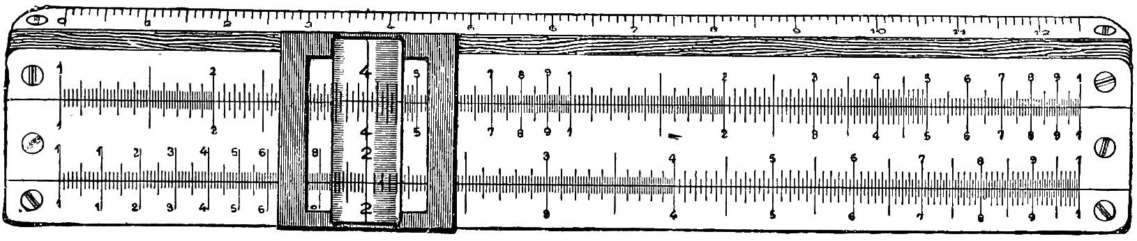
From Fig. 5, which is a representation
of the face of a Gravêt or Mannheim slide
rule, it will be seen that four series of logarithmic
graduations or scale-lines are employed,
the upper and lower being engraved
on the stock or body of the rule, while the
other two are engraved upon the slide. The
two upper sets of graduations are exactly
alike in every particular, and the lower
sets are also similar. It is usual to identify
the two upper scale-lines by the letters A
and B, and the two lower by the letters C
and D, as indicated in the figure at the
left-hand extremities of the scales.
Referring to the scales C and D, these
will each be seen to be a development
of the elementary scales of Fig. 3, but
13in this case each principal space is subdivided, more or
less minutely. The principle, however, is exactly the same,
so that by moving the slide (carrying scale C), multiplication
and division can be mechanically performed in the manner
described.
The upper scale-line A consists of two exactly similar scales,
placed end to end, the first lying between Il and Ic, and the
second between Ic and Ir. The first of these scales will be designated
the left-hand A scale, and the second the right-hand A scale.
Similarly the coinciding scales on the slide are the left-hand B
scale and the right-hand B scale. Each of these four scales is
divided (as finely as convenient) as in the case of the C and D
scales, but, of course, they are exactly one half the length of the
latter.
The two end graduations of both the C and D scales are known
as the left- and right-hand indices of these scales. Sometimes they
are figured 1 and 10 respectively; sometimes both are marked 1.
Similarly Il and Ir are the left- and right-hand indices of the A
and B lines, while Ic is the centre index of these scales. Other
division lines usually found on the face of the rule are one on the
left-hand A and B scales, indicating the ratio of the circumference
of a circle to its diameter, π = 3·1416; and a line on the right-hand
B scale marking the position of π 4 = 0·7854, used in calculating
the areas of circles. Reference will be made hereafter to the
scales on the under-side of the slide, and we need now only add
that one of the edges of the rule, usually bevelled, is generally
graduated in millimetres, while the other edge has engraved on it
a scale of inches divided into eighths or tenths. On the bottom
face inside the groove of the rule either one or the other of these
scales is continued in such a manner that by drawing the slide out
to the right and using the scale inside the rule, in conjunction
with the corresponding scale on the edge, it is possible to measure
20 inches in the one case, or nearly 500 millimetres in the other.
On the back of the rule there is usually a collection of data, for
which the slips given at the end of this work may often be substituted
with advantage.
THE NOTATION OF THE SLIDE RULE.
14
Hitherto our attention has been confined to a consideration of
the primary divisions of the scales. The same principle of graduation
is, however, used throughout; and after what has been said,
this part of the subject need not be further enlarged upon. Some
explanation of the method of reading the scales is necessary, as
facility in using the instrument depends in a very great measure
upon the dexterity of the operator in assigning the correct value
to each division on the rule. By reference to Fig. 5, it will be
seen that each of the primary spacings in the several scales is
invariably subdivided into ten; but since the lengths of the
successive primary divisions rapidly diminish, it is impossible to
subdivide each main space into the same number of parts that
the space 1–2 can be subdivided. This variable spacing of the
scales is at first confusing to the student, but with a little practice
the difficulty is soon overcome.
With the C or D scale, it will be noticed that the length of the
interval 1–2 is sufficient to allow each of the 10 subdivisions to be
again divided into 10 parts, so that the whole interval 1–2 is
divided into 100. The shorter main space 2–3, and the still shorter
one 3–4, only allow of the 10 subdivisions of each being divided
into five parts. Each of these main spaces is therefore divided
into 50 parts. For the remainder of the scale each of the 10
subdivisions of each main space is divided into two parts only; so
that from the main division 4 to the end of the scale the primary
spaces are divided into 20 parts only.
In the upper scales A or B, it will be found that—as the space
1–2 is of only half the length of the corresponding space on C or D—the
10 subdivisions of this interval are divided into five parts
only. Similarly each of the 10 subdivisions of the intervals 2–3,
3–4, and 4–5 are further divided into two parts only, while
for the remainder of the scale only the 10 subdivisions are
possible, owing to the rapidly diminishing lengths of the primary
spacings.
The values actually given on the rule run from 1 to 10 on
the lower scales and from 1 to 100 on the upper scales, and, as
explained on page 9, all factors are brought within these ranges
of values by multiplying or dividing them by powers of 10. By
following this plan, we virtually regard each factor as merely a
15series of significant figures, and make the necessary modification
due to the “powers of 10” when fixing the position of the decimal
point in the answer.
Many, however, find it convenient in practice to regard the
values on the rule as multiplied or divided by such powers of 10
as may be necessary to suit the factors entering into the calculation.
If this plan is adopted, the values given to each graduation
of the scales will depend on that given to the left index figure (1)
of the lower scales, this being any multiple or submultiple of 10.
Thus Il on the D scale may be regarded as 1, 10, 100, 1000, etc., or
as 0·1, 0·01, 0·001, 0·0001, etc.; but once the initial value is assigned
to the index, the ratio of value must be maintained throughout the
whole scale. For example, if 1 on C is taken to represent 10, the
main divisions 2, 3, 4, etc., will be read as 20, 30, 40, etc. On
the other hand, if the fourth main division is read as 0·004, then
the left index figure of the scale will be read as 0·001. The figured
subdivisions of the main space 1–2 are to be read as 11, 12, 13, 14,
15, 16, 17, 18 and 19—if the index represents 10,—and as corresponding
multiples for any other value of the index.
Independently considered, these remarks apply equally to the
A or B scale, but in this case the notation is continued through
the second half of the scale, the figures of which are to be read as
tenfold values of the corresponding figures in the first half of the
scale.
The reading of the intermediate divisions will, of course, be
determined by the values assigned to the main divisions. Thus, if
Il on D is read as 1, then each of the smallest subdivisions of the
space 1–2 will be read as 0·01, and each of the smallest subdivisions
of the spaces 2–3 or 3–4 as 0·02, while for the remainder of the
scale the smallest subdivisions are read as 0·05. In the A or B
scale the subdivisions of the space 1–2 of the first half of the scale
are (if Il = 1) read as 0·02, 0·04, etc.; for the divisions 2–3, 3–4, and
4–5, the smallest intervals are read as 0·05 of the primary spaces,
and from 5 to the centre index of the scale the divisions represent
0·1 of each main interval. Passing the centre index, which is, now
read as 10, the smallest subdivisions immediately following are
read 10·2, 10·4, etc., until 20·0 is reached; then we read 20·5, 21·0,
21·5 22·0, etc., until the figured main division 5 is reached. The
remainder of the scale is read 51, 52, 53, etc., up to 100, the right-hand
index.
16Further subdivision of any of the spaces of the rule can be
effected by the eye, and after a little practice the operator will
become quite expert in estimating any intermediate value. It
affords good practice to set 1 on C to 1·04, 1·09, etc. on D, and to
read the values on D, under 4, 6, 8, etc. on C. As the exact
results are easily calculated mentally, the student, by this means,
will receive better instruction in estimating intermediate results
than can be given by any diagram.
Some rules will be found figured as shown in Fig. 5; in others,
the right-hand upper scales are marked 10, 20, 30, etc. Again,
others are marked decimally, the lower scales and the left-hand
upper scales being figured 1, 1·1, 1·2, 1·3 ... 2·5, etc. The
latter form has advantages from the point of view of the
beginner.
The method of reading the A and B scales, just given, applies
only when these scales are regarded as altogether independent of
the lower pair of scales C and D. Some operators prefer to use
the A and B scales, and some the C and D scales, for the ordinary
operations of proportion, multiplication, and division. Each
method has its advantages, as will be shown, but in the more
complex calculations, as involution and evolution, etc., the relation
of the upper scales to the lower scales becomes a very important
factor.
The distance 1–10 on the upper scales is one-half of the distance
1–10 on the lower scales. Hence any distance from 1, taken on
the upper scales, represents twice the logarithm which the same
distance represents on the lower scales. In other words, the length
which represents log. N on D, would represent 2 log. N on A;
and, conversely, the length which represents log. N on A, would
represent log. N 2 on D.
Now we have seen (page 8) that multiplying the log. of a
number by 2 gives the log. of the square of the number. Hence,
above any number on D we find its square on A, or, conversely,
below any number on A, we find its square root on D. Thus,
above 2 we find 4; under 49, we find 7 and so on. Obviously the
same relation exists between the B and C scales.
THE CURSOR OR RUNNER.
17
All modern slide rules are now fitted with a cursor or runner,
which usually consists of a light metal frame moving under spring
control in grooves in the edges of the stock of the rule. This
frame carries a piece of glass, mica or transparent celluloid, about
1 in. square, across the centre of which a fine reference line is
drawn exactly at right angles to the line of scales. To “set the
cursor” to any value on the scales of the rule, the frame is taken
between the thumb and forefinger and adjusted in position until
the line falls exactly upon the graduation, or upon an estimated
value, between a pair of graduations, as the case may be. Having
fixed one number in this way, another value on either of the scales
on the slide may be similarly adjusted in reference to the cursor
line. The cursor will be found very convenient in making such
settings, especially when either or both of the numbers are located
by eye estimation. It also finds a very important use in referring
the readings of the upper scale to those of the lower, or vice versa,
while as an aid in continued multiplication and division and complex
calculations generally, its value is inestimable.
Multiple Line Cursors.—Cursors can be obtained with two lines,
the distance between them being that between 7·854 and 10 on
the A scale. The use of this cursor is explained on page 57.
Another multiple line cursor has short lines engraved on it, corresponding
to the main graduations from 95 to 105 on the respective
scales. This is useful for adding or deducting small percentages.
The Broken Line Cursor.—To facilitate setting, broken line
cursors are made, in which the hair-line is not continued across
the scales, but has two gaps, as shown in Fig. 6.
The Pointed Cursor has an index or pointer, extending over the
bevelled edge of the rule, on which is a scale of inches. It is
useful for summing the lengths of the ordinates of indicator
diagrams, and also for plotting lengths representing the logarithms
of numbers, sometimes required in graphic calculations.
The Goulding Cursor.—It has been pointed out that in order to
obtain the third or fourth figure of a reading on the 10 in. slide
rule, it is frequently necessary to depend upon the operator’s
ability to mentally subdivide the space within which the reading
falls. This subdivision can be mechanically effected by the aid of
the Goulding Cursor (Fig. 7), which consists of a frame fitting
18into the usual grooves in the rule, and carrying a metal plate faced
with celluloid, upon which is engraved a triangular scale A B C.
The portion carrying the chisel edges E is not fixed to the cursor
proper, but slides on the latter, so that the index marks on the
projecting prongs can be moved slightly along the scales of the
rule, this movement being effected by the short end of the bent
lever F working in the slot as shown. D is a pointer which can
be moved along F under spring control. As illustrating the
method of use, we will assume that 1 on C is placed to 155 on D,
and that we require to read the value on D under 27 on C. This
is seen to lie between 4150 and 4200, so setting the pointer D to
the line B C—always the first operation—we move the whole
along the rule until the index line on the lower prong agrees with
4200. We then move F across the scale until the index line agrees
with 4100, set the pointer D to the line A C, and move the lever
back until the index line agrees with 27 on the slide. It will then
be found that the pointer D gives 85 on A B as the value of the
supplementary figures, and hence the complete reading is 4185.
Fig. 6.
Fig. 8.
Fig. 7.
Fig. 9.
Magnifying Cursors are of assistance in reading the scales, and
in a good and direct light are very helpful. In one form an
ordinary lens is carried by two light arms hinged to the upper
and lower edges of the cursor, so that it can be folded down to the
face of the rule when not in use. A more compact form, shown in
19Fig. 8, consists of a strip of plano-convex glass, on the under-side
of which is the hair-line. In a cursor made by Nestler of Lahr,
the plano-convex strip is fixed on the ordinary cursor. The
magnifying power is about 2, so that a 5 in. rule, having the same
number of graduations as a 10 in. rule, can be read with equal
facility, by the aid of this cursor.
The Digit-registering Cursor, supplied by Mr. A. W. Faber,
London, and shown in Fig. 9, has a semicircular scale running
from 0 at the centre upward to −6 and downward to +6. A
small finger enables the operator to register the number of digits
to be added or subtracted at the end of a lengthy operation, as
explained at page 28.
MULTIPLICATION.
In the preliminary notes it was shown that by mechanically
adding two lengths representing the logarithms of two numbers, we
can obtain the product of these numbers; while by subtracting one
log. length from another, the number represented by the latter is
divided by the number represented by the former. Hence, using
the C and D scales, we have the
Rule for Multiplication.—Set the index of the C scale to one of the
factors on D, and under the other factor on C, find the product on D.
Fig. 10.
Thus, to find the product of 2 × 4, the slide is moved to the right
until the left index (1) of C is brought over 2 on D, when under the
other factor (4) on C, is found the required product (8) on D.
Following along the slide, to the right, we find that beyond 5 on C
(giving 10 on D), we have no scale below the projecting slide (Fig.
10). If we imagine the D scale prolonged to the right, we should
have a repetition of the earlier portion, but, as with the two parts
20of the A scales, the repeated portion would be of tenfold value, and
10 on C would agree with 20 on the prolonged D scale. We turn
this fact to account by moving the slide to the left until 10 on C
agrees with 2 on D, and we can then read off such results as
2 × 6 = 12; 2 × 8 = 16, etc., remembering that as the scale is now of
tenfold value, there will be two figures in the result. Hence, for
those who prefer rules, we have the
Rule for the Number of Digits in a Product.—If the product
is read with the slide projecting to theLEFT, ADD THE NUMBER
OF THE DIGITS IN THE TWO FACTORS; if read with the slide to theRIGHT, deduct 1 from this sum.
Ex.—25 × 70 = 1750.
The product is found with the slide projecting to the left, so
the number of digits in the product = 2 + 2 = 4.
Ex.—3·6 × 25 = 90.
The slide projects to the right, and the number of digits in the
product is therefore 1 + 2 − 1 = 2.
Ex.—0·025 × 0·7 = 0·0175.
The product is obtained with the slide projecting to the left,
and the number of digits is therefore −1 + 0 = −1.
Ex.—0·000184 × 0·005 = 0·00000092.
The sum of the number of digits in the two factors = −3 + (−2)
= −5, but as the slide projects to the right, the number of digits
will be −5 − 1 = −6.
From the last two examples it will be seen that when the first
significant figure of a decimal factor does not immediately follow
the decimal point, the minus sign is to be prefixed to the number
of digits, counting as many digits minus as there are 0’s following
the decimal point. Thus, 0·03 has −1 digit, 0·0035 has −2 digits,
and so on. Some little care is necessary to ensure these minus
values being correctly taken into account in determining the
number of digits in the answer. For this reason many prefer to
treat decimal factors as whole numbers, and to locate the decimal
point according to the usual rules for the multiplication of decimals.
Thus, in the last example we take 184 × 5 = 920, but as by the usual
rule the product must contain 6 + 3 = 9 decimal places, we prefix
six cyphers, obtaining 0·00000092. When both factors consist of
integers as well as decimals, the number of digits in the product,
and therefore the position of the decimal point, will be determined
by the usual rule for whole numbers.
21Another method of determining the number of digits in a
product deserves mention, which, not being dependent upon the
position of the slide, is applicable to all calculating instruments.
General Rule for Number of Digits in a Product.—When
the first significant figure in the product is smaller than inEITHERof
the factors, the number of digits in the product is equal to theSUMof
the digits in the two factors. When the contrary is the case, the
number of digits is 1LESSthan the sum of the digits in the two
factors. When the first figures are the same, those following must be
compared.
Estimation of the Figures in a Product.—We have given rules for
those who prefer to decide the number of figures by this means,
but experience will show that to make the best use of the instrument,
the result, as read on the rule, should be regarded merely
as the significant figures of the answer, the position of the decimal
point, if not obvious, being decided by a very rough mental calculation.
In very many instances, the magnitude of the result will
be evident from the conditions of the problem—e.g., whether the
answer should be 0·3 in., 3 in., or 30 in.; or 10 tons, 0·1 ton, 100
tons, etc. In those cases where the magnitude of the answer cannot
be estimated, and the factors contain many figures, or have a
number of 0’s following the decimal point, the use of notation by
powers of 10 (page 8) is of considerable assistance; but more
usually it will be found, that a very rough calculation will settle the
point with comparatively little trouble. Considerable practice is
needed to work rapidly and with certainty, when using rules.
Moreover, the experience thus acquired is confined to slide-rule
work. The same time spent in practising the “rough approximation”
method will enable reliable results to be obtained
rapidly, with the advantage that the method is applicable to
calculations generally. However, the choice of methods is a
matter of personal preference. Both methods will be given, but
whichever plan is followed, the student is strongly advised to
cultivate the habit of forming an idea of the magnitude of the
result.
Ex.—33·6 × 236 = 7930.
Setting 1 on C to 33·6 on D, we read under 236 on D and find 793
on D, as the significant figures of the answer. A rough calculation,
as 30 × 200 = 6000, indicates that the result will consist of 4 figures,
and is therefore to be read as 7930.
22Ex.—17,300 × 3780 = 65,400,000.
By factorising with powers of 10
1·73 × 104 × 3·78 × 103 = 1·73 × 3·78 × 107.
Setting 1 on C to 1·73 on D, we read, under 3·78 on C, the result
of the simple multiplication, as 6·54. Multiplying by 107 moves the
decimal point 7 places to the right, and the answer is 65,400,000.
If it is required to find a series of products of which one of the
factors is constant, set 1 on C to the constant factor on D and read
the several products on D, under the respective variable factors.
If the factors are required which will give a constant product
(really a case of division), set the cursor to the constant product on
D. Then obviously, as the slide is moved along, any pair of factors
found simultaneously under the cursor line on C, and on D under
index of C, will give the product. A better method of working
will be explained when we deal with the inversion of the slide.
It is sometimes useful to remember that although we usually
set the slide to the rule, we can obtain the result equally well by
setting the rule to the slide. Thus, bringing 1 (or 10) on D to 2
on C, we find on C, over any other factor, n on D, the product of
2 × n. But note that the slide and rule have now changed places,
and if we use rules for the number of digits in the result, we
must now deduct 1 from the sum of the digits in the factors,
when the rule projects to the right of the slide.
With the ordinary 10 in. rule it will be found in general that
the extent to which the C and D scales are subdivided is such as
to enable not more than three figures in either factor being dealt
with. For the same reason it is impossible to directly read more
than the first three figures of any product, although it is often
possible—by mentally dividing the smallest space involved in the
reading—to correctly determine the fourth figure of a product.
Necessarily this method is only reliable when used in the earlier
parts of the C and D scales. However, the last numeral of a
three-figure, and in some cases the last of a four-figure, product
can be readily ascertained by an inspection of the factors.
Ex.—19 × 27 = 513. Placing the L.H. index of C to 19 on D,
we find opposite 27 on C, the product, which lies between 510 and
515. A glance at the factors, however, is sufficient to decide that
the third figure must be 3, since the product of 9 and 7 is 63, and
the last figure of this product must be the last figure in the answer.
Ex.—79 × 91 = 7189.
23In this case the division line 91 on C indicates on D that the
answer lies between 7180 and 7190. As the last figure must be 9,
it is at once inferred that the last two figures are 89.
When there are more than three figures in either or both of the
factors, the fourth and following figures to the right must be
neglected. It is well to note, however, that if the first neglected
figure is 5, or greater than 5, it will generally be advisable to
increase by 1 the third figure of the factor employed. Generally
it will suffice to make this increase in one of the two factors only,
but it is obvious that in some cases greater accuracy will be
obtained by increasing both factors in this way.
Continued Multiplication.—To find the product of more
than two factors, we make use of the cursor to mark the position
of successive products (the value of which does not concern us) as
the several factors are taken into the calculation. Setting the index
of C to the 1st factor on D, we bring the line of the cursor to the
2nd factor on C, then the index of C to the cursor, the cursor to
the 3rd factor, index of C to cursor, and so on, reading the final product
on D under the last factor on C. (Note that the 1st factor and
the result are read on D; all intermediate readings are taken on C.)
If the rule for the number of digits in a product is used, it is
necessary to note the number of times multiplication is effected
with the slide projecting to the right. This number, deducted
from the sum of the digits of the several factors, gives the number
of digits in the product. Ingenious devices have been adopted to
record the number of times the slide projects to the right, but
some of these are very inconvenient. The author’s method is to
record each time the slide so projects, by a minus mark, thus −.
These can be noted down in any convenient manner, and the sum
of the marks so obtained deducted from the sum of the digits in
the several factors, gives the number of digits in the product as
before explained.
Ex.—42 × 71 × 1·5 × 0·32 × 121 = 173,200.
The product given, which is that read on the rule, is obtained
as follows:—Set R.H. index of C to 42 on D, and bring the cursor
to 71 on C. Next bring the L.H. index of C to the cursor, and the
latter to 1·5 on C. This multiplication is effected with the slide
to the right, and a memorandum of this fact is kept by making a
mark −. Bring the R.H. index of C to the cursor and the latter to
0·32 on C. Then set the L.H. index of C to the cursor and read
24the result, 1732, on D under 121 on C, while as a slide again
projects to the right, a second − memo-mark is recorded. There
are 2 + 2 + 1 + 0 + 3 = 8 digits in the factors, and as there were 2 −
marks recorded during the operation, there will be 8 − 2 = 6 digits
in the product, which will therefore read 173,200 (173,194·56).
For a very rough evaluation of the result, we note that 1·5 × 0·3
is about 0·5; hence, as a clue to the number of figures we have
40 × 70 × 60 = 3000 × 60 = 180,000.
DIVISION.
The instructions for multiplication having been given in some detail,
a full discussion of the inverse process of division will be unnecessary.
Rule for Division.—Place the divisor on C, opposite the dividend
on D, and read the quotient on D under the index of C.
Ex.—225 ÷ 18 = 12·5.
Bringing 18 on C to 225 on D, we find 12·5 under the L.H.
index of C.
As in multiplication, the factors are treated as whole numbers,
and the position of the decimal point afterwards decided according
to the following rule, which, as will be seen, is the reverse of that
for multiplication:—
Rule for the Number of Digits in a Quotient.—If the
quotient is read with the slide projecting to theLEFT, subtract the
number of digits in the divisor from those in the dividend; but if
read with the slide to theRIGHT, ADD1 to this difference.[2]
In the above example the quotient is read off with the slide to
the right, so the number of digits in the answer = 3 − 2 + 1 = 2.
Ex.—0·000221 ÷ 0·017 = 0·013.
Here the number of digits in the dividend is −3, and in the divisor
−1. The difference is −2; but as the result is obtained with the
slide to the right, this result must be increased by 1, so that the number
of digits in the quotient is −2 + 1 = −1, giving the answer as 0·013.
If preferred, the result can be obtained in the manner referred
to when considering the multiplication of decimals. Thus, treating
the above as whole numbers, we find that the result of dividing
221 by 17 = 13, since the difference in the number of digits in the
factors, which is 1, is, owing to the position of the slide, increased
by 1, giving 2 as the number of digits in the answer. Then by the
25rules for the division of decimals we know that the number of
decimal places in the quotient is equal to 6 − 3 = 3, showing that a
cypher is to be prefixed to the result read on the rule.
As in multiplication, so in division, we have a
General Rule for Number of Digits in a Quotient.—When
the first significant figure in theDIVISORis greater than that in theDIVIDEND, the number of digits in the quotient is found by subtracting
the digits in the divisor from those in the dividend. When the contrary
is the case, 1IS TO BE ADDEDto this difference. When the first figures
are the same, those following must be compared.
Estimation of the Figures in a Quotient.—The method of
roughly estimating the number of figures in a quotient needs little
explanation.
Ex.—3·95 ÷ 5340 = 0·00074.
Setting 534 on C to 3·95 on D we read under the (R.H.) index of
C, the significant figures on D, which are 74. Then 3·9 ÷ 5 is about 0·8
and 0·8 ÷ 1000 gives 0·0008 as a rough estimate.
Ex.—0·00000285 ÷ 0·000197 = 0·01446.
Regarding this as 2·85 × 10−6 ÷ 1·97 × 10−4 we divide 2·85 by 1·97
and obtain 1·446. Dividing the powers of 10 we have 10−6 ÷ 10−4 =
10−2, so the decimal point is to be moved two places to the left and the
answer is read as 0·01446.
Another method of dividing deserves mention as of special
service when dividing a number of quantities by a constant divisor:—Set
the index of C to the divisor on D and over any dividend on D,
read the quotient on C.
For the division of a constant dividend by a variable divisor,
set the cursor to the dividend on D and bring the divisor on C
successively to the cursor, reading the corresponding quotients on
D under the index of C. Another method which avoids moving
the slide is explained in the section on “Multiplication and Division
with the Slide Inverted.”
Continued Division, if we can so call such an expression as
3·14 785 × 0·00021 × 4·3 × 64·4 = 0·0688,
may be worked by repeating as follows:—Set 7·85 on C to 3·14 on
D, bring cursor to index of C, 2·1 on C to cursor, cursor to index,
4·3 to cursor, cursor to index, 6·44 to cursor, and under index of C
read 688 on D as the significant figures of the answer.
For the number of figures in the result, we deduct the sum of
the number of digits in the several factors and add 1 for each
26time the slide projects to the right, which in this case occurs once.
There are 3 + (−3) + 1 + 2 = 3 denominator digits, 1 numerator digit,
and 1 is to be added to the difference. Therefore there are
1 − 3 + 1 = −1 digits in the answer, which is therefore 0·0688. The
foregoing method of working may confuse the beginner, who is apt
to fall into the process of continued multiplication. For this
reason, until familiarity with combined methods has been acquired,
the product of the several denominators should be first found by
the continued multiplication process, and the figures in this product
determined. Then divide the numerator by this product to obtain
the result.
As the denominator product will be read on D, we may avoid
resetting the slide by bringing the numerator on C to this product
and reading the result on C over the index of D. The slide and
rule have here changed places; hence if rules are followed for the
number of figures in the result, 1 must be added to the difference
of digits, when the rule projects to the right of the slide.
The author’s method of recording the number of times division
is performed with the slide to the right is by vertical memorandum
marks, thus |. The full significance of these memo-marks will
appear in the following section.
For a rough calculation to fix the decimal point, in this example
we move the decimal points in the factors, obtaining
3 0·8 × 2 × 4 × 6 = 3 40 = 0·075.
THE USE OF THE UPPER SCALES FOR MULTIPLICATION AND DIVISION.
Many prefer to use the upper scales A and B, in preference to C
and D. The disadvantage is that as the scales are only one-half
the length of C or D, the graduation does not permit of the same
degree of accuracy being obtained as when working with the lower
scales. But the result can always be read directly from the rule
without ever having to change the position of the slide after it has
been initially set. Hence, it obviates the uncertainty as to the
direction in which the slide is to be moved in making a setting.
When the A and B scales are employed, it is understood that
the left-hand pair of scales are to be used in the same manner as
C and D, and so far the rules relating to the latter are entirely
applicable. But in this case the slide is always moved to the
27right, so that in multiplication the product is found either upon
the left or right scales of A. If it is found on the left A scale,
the rule for the number of digits in the product is found as for
the C and D scales, and is equal to the sum of the digits in the two
factors, minus 1; but if found on the right-hand A scale, the
number of digits in the product is equal to the sum of the digits
in the two factors.
In division, similar modifications are necessary. If when
moving the slide to the right the division can be completely
effected by using the L.H. scale of A, the quotient (read on A above
the L.H. of index B) has a number of digits equal to the number in
the dividend, less the number in the divisor, plus 1. But if the
division necessitates the use of both the A scales, the number of
digits in the quotient equals the number in the dividend, less the
number in the divisor.
RECIPROCALS.
A special case of division to be considered is the determination of
the reciprocal of a number n, or 1 n. Following the ordinary rule for
division, it is evident that setting n on C to 1 on D, gives 1 n on D
under 1 on C. It is more important to observe that by inverting
the operation—setting 1 (or 10) on C to n on D—we can read 1 n on
C over 1 (or 10) on D. Hence whenever a result is read on D
under an index of C, we can also read its reciprocal on C over
whichever index of D is available.
The Number of Digits in a Reciprocal is obvious when n = 10,
100, or any power (p) of 10. Thus 1 10 = 0·1; 1 100 = 0·01; 1 10p = 1
preceded by p − 1 cyphers. For all other cases we have the rule:—Subtract
from 1 the number of digits in the number.
Ex.—1 339 = 0·00295.
There are 3 digits in the number; hence, there are 1 − 3 = −2
digits in the answer.
Ex.—1 0·0000156 = 64,100.
There are −4 digits in the number; hence, there are 1 − (−4) = 5
digits in the result.
CONTINUED MULTIPLICATION AND DIVISION.
28
By combining the rules for multiplication and division, we can
readily evaluate expressions of the form a b × c d × e f × g h = x. The
simplest case, a × c b can be solved by one setting of the slide.[3]
Take as an example, 14·45 × 60 8·5 = 102. Setting 8·5 on C to 14·45 on
D, we can, if desired, read 1·7 on D under 1 on C, as the quotient.
However, we are not concerned with this, but require its multiplication
by 60, and the slide being already set for this operation, we
at once read under 60 on C the result, 102, on D. The figures in
the answer are obvious.
When there are more factors to take into account, we place the
cursor over 102 on D, bring the next divisor on C to the cursor,
move the cursor to the next multiplier on C, bring the next divisor
on C to the cursor, and so on, until all the factors have been dealt
with. Note that only the first factor and the result are read on
D; also that the cursor is moved for multiplying and the slide for
dividing.
Number of Digits in Result in Combined Multiplication and
Division.—For those who use rules the author’s method of determining
the decimal point in combined multiplication and division
may be used. Each time multiplication is performed with the slide
projecting to the right, make a − mark; each time division is
effected with the slide to the right, make a | mark; but allow
the | marks to cancel the − marks as far as they will. Subtract
the sum of the digits in the denominator from the sum of digits in
the numerator, and to this difference add any uncancelled memo-marks,
if of | character, or subtract them if of − character.
Set 27 on C to 43·5 on D, and as with this division the
slide is to the right, make the first ⵏ mark. Bring cursor
to 29·4 on C, and as in this multiplication the slide is to
the right, make the first − mark, cancelling as shown.
29Setting 3·83 on C to the cursor, requires the
second ⵏ mark, which, however, is cancelled in
turn by the multiplication by 51. The division
by 10·5 requires the third ⵏ mark, and after multiplying
by 32 (requiring no mark) the final division
by 1·31 requires the fourth ⵏ mark. Then, as there
are 8 numerator digits, 6 denominator, and 2 uncancelled
memo-marks (which, being 1, are additive)
we have
Number of digits in result = 8 − 6 + 2 = 4.
Had the uncancelled marks been − in character, the number of
digits would have been 8 − 6 − 2 = 0.
For quantities less than 0·1 the digit place numbers will be
negative. The troublesome addition of these may be avoided by
transferring them to the opposite side and treating them as
positive.
2
4
Thus:—
0·00356
×
27·1
×
0·08375
= 288
0·1426
×
9·85
×
0·00002
2
1
1
The first numerator, 0·00356, has −2 digits. Note this by
placing 2 below the lower line as shown. 27·1 has 2 digits; place 2
over it. 0·08375 has −1 digit; hence place 1 below the lower line.
The first denominator has no digits; the second, 9·85, has 1 digit;
hence place 1 under it. 0·00002 has −4 digits; place 4 above the
upper line. The sum of the top series is 2 + 4 = 6; of the bottom
series 2 + 1 + 1 = 4. Subtracting the bottom from the top, we have
6 − 4 = 2 digits, to which 1 has to be added for an uncancelled
memo-mark, and the result is read as 288.
Moving the decimal point often facilitates matters. Thus,
32·4 × 0·98 × 432 × 0·0217 4·71 × 0·175 × 0·00000621 × 412000 is much more conveniently dealt
with when re-arranged as 32·4 × 9·8 × 432 × 2·17 4·71 × 17·5 × 6·21 × 4·12 = 141.
To determine the number of figures in the result by rough
cancelling and mental calculation, we note that 4·71 enters 432
about 100 times; 9·8 enters 17·5 about 2; 6·21 into 32·4 about 5;
and 2·17 into 4·12 about 2. This gives 500 4 = 125, showing that
the result contains 3 digits. From the slide rule we read 141,
which is therefore the result sought.
30The occasional traversing of the slide through the rule, to
interchange the indices—a contingency which the use of the C and
D scales always involves—may often be avoided by a very simple
expedient. Such an example as 6·19 × 31·2 × 422 1120 × 8·86 × 2.09 = 3·93 is sometimes
cited as a particularly difficult case. Working through the
expression as given, two traversings of the slide are necessary;
but by taking the factors in the slightly different order,
6·19 × 31·2 × 422 8·86 × 2·09 × 1120, so that the significant figures of each pair are more
nearly alike, we not only avoid any traversing the slide, but we
also reduce the extent to which the slide is moved to effect the
several divisions.
Such cases as a × b c × d × e × f × g or a × b × c × d × e f × g really resolve
themselves into a × b × 1 × 1 × 1 c × d × e × f × g and a × b × c × d × e f × g × 1 × 1 × 1, but, of course,
if rules are used to locate the decimal point, the 1’s so (mentally) introduced
are not to be counted as additional figures in the factors.
MULTIPLICATION AND DIVISION WITH THE SLIDE INVERTED.
If the slide be inverted in the rule but with the same face
uppermost, so that the Ɔ scale lies adjacent to the A scale, and the
right and left indices of the slide and rule are placed in coincidence,
we find the product of any number on D by the coincident number
on Ɔ (readily referred to each other by the cursor) is always 10.
Hence, by reading the numbers on Ɔ as decimals, we have over
any unit number on D, its reciprocal on Ɔ. Thus 2 on D is found
opposite 0·5 on Ɔ; 3 on D opposite to 0·333; while opposite 8 on
Ɔ is 0·125 on D, etc. The reason of this is that the sum of the
lengths of the slide and rule corresponding to the factors, is
always equal to the length corresponding to the product—in this
case, 10.
It will be seen that if we attempt to apply the ordinary rule
for multiplication, with the slide inverted, we shall actually be
multiplying the one factor taken on D by the reciprocal of the
other taken on Ɔ. But multiplying by the reciprocal of a number
is equivalent to dividing by that number, and dividing a factor by
the reciprocal of a number is equivalent to multiplying by that
31number. It follows that with the slide inverted the operations of
multiplication and division are reversed, as are also the rules for
the number of digits in the product and the position of the decimal
point. Hence, in multiplying with the slide inverted, we place
(by the aid of the cursor) one factor on Ɔ opposite the other factor
on D, and read the result on D under either index of Ɔ. It follows
that with the slide thus set, any pair of coinciding factors on Ɔ
and D will give the same constant product found on D under the
index of Ɔ. One useful application of this fact is found in selecting
the scantlings of rectangular sections of given areas or in
deciding upon the dimensions of rectangular sheets, plates, cisterns,
etc. Thus by placing the index of Ɔ to 72 on D, it is readily seen
that a plate having an area of 72 sq. ft. may have sides 8 by 9 ft.,
6 by 12, 5 by 14·4, 4 by 18, 3 by 24, 2 by 36, with innumerable
intermediate values. Many other useful applications of a similar
character will suggest themselves.
PROPORTION. — GENERAL HINTS ON THE ELEMENTARY USES OF THE SLIDE RULE. — SQUARES AND SQUARE ROOTS. — CUBES AND CUBE ROOTS. — MISCELLANEOUS POWERS AND ROOTS. — POWERS AND ROOTS BY LOGARITHMS.
With the slide in the ordinary position and with the indices of
the C and D scales in exact agreement, the ratio of the corresponding
divisions of these scales is 1. If the slide is moved so that
1 on C agrees with 2 on D, we know that under any number n on
C is n × 2 on D, so that if we read numerators on C and denominators
on D we have
C
1
1·5
2
3
4
D1
2
3
4
6
8.
In other words, the numbers on D bear to the coinciding numbers
on C a ratio of 2 to 1. Obviously the same condition will obtain
no matter in what position the slide may be placed. The rule for
proportion, which is apparent from the foregoing, may be expressed
as follows:—
Rule for Proportion.—Set the first term of a proportion on the
C scale to the second term on the D scale, and opposite the third term
on the C scale read the fourth term on the D scale.
Ex.—Find the 4th term in the proportion of 20 ∶ 27 ∷ 70 ∶ x.
Set 20 on C to 27 on D, and opposite 70 on C read 94·5 on D. Thus
C
20
70
D
27
94·5.
It will be evident that this is merely a case of combined
multiplication and division of the form, 20 × 70 27 = 94·5. Hence,
32given any three terms of a proportion, we set the 1st to the 2nd,
or the 3rd to the 4th, as the case may be, and opposite the other
given term read the term required.[4]
Thus, in reducing vulgar fractions to decimals, the decimal
equivalent of 3 16 is determined by placing 3 on C to 16 on D, when
over the index or 1 of D we read 0·1875 on C. In this case the
terms are 3 ∶ 16 ∷ x ∶ 1. For the inverse operation—to find a
vulgar fraction equivalent to a given decimal—the given decimal
fraction on C is set to the index of D, and then opposite any
denominator on D is the corresponding numerator of the fraction
on C.
If the index of C be placed to agree with 3·1416 on D, it will
be clear from what has been said that this ratio exists throughout
between the numbers of the two scales. Therefore, against any
diameter of a circle on C will be found the corresponding circumference
on D. In the same way, by setting 1 on C to the appropriate
conversion factor on D, we can convert a series of values in one
denomination to their equivalents in another denomination. In
this connection the following table of conversion factors will be
found of service. If the A and B scales are used instead of the
C and D scales, a complete set of conversions will be at once
obtained. In this case, however, the left-hand A and B scales
should be used for the initial setting, any values read on the right-hand
A or B scales being read as of tenfold value. With the C and
D scales a portion of the one scale will project beyond the other.
To read this portion of the scale, the cursor or runner is brought
to whichever index of the C scale falls within the rule, and the
slide moved until the other index of the C scale coincides with
the cursor, when the remainder of the equivalent values can then
be read off. It must be remembered that if the slide is moved in
the direction of notation (to the right), the values read thereon
have a tenfold greater value; if the slide is moved to the left, the
readings thereon are decreased in a tenfold degree. Although
preferred by many, in the form given, the case is obviously one of
multiplication, and is so treated in the Data Slips at the end of
the book.
33
TABLE OF CONVERSION FACTORS.
Geometrical Equivalents.
Scale C.
Scale D.
If C = 1, D =
Diameter of circle
Circumference of circle
3·1416
„ „
Side of inscribed square
0·707
„ „
„ equal square
0·886
„ „
„ „ equilateral triangle
1·346
Circum. of circle
„ inscribed square
0·225
„ „
„ equal square
0·282
Side of square
Diagonal of square
1·414
Square inch
Circular inch
1·273
Area of circle
Area of inscribed square
0·636
Measures of Length.
Inches
Millimetres
25·40
„
Centimetres
2·54
8ths of an inch
Millimetres
3·175
16ths „ „
„
1·587
32nds „ „
„
0·794
64ths „ „
„
0·397
Feet
Metres
0·3048
Yards
„
0·9144
Chains
„
20·116
Miles
Kilometres
1·609
Measures of Area.
Square inches
Square centimetres
6·46
Circular „
„ „
5·067
Square feet
„ metres
0·0929
„ yards
„ „
0·836
„ miles
„ kilometres
2·59
„ „
Hectares
259·00
Acres
„
0·4046
Measures of Capacity.
Cubic inches
Cubic centimetres
16·38
„ „
Imperial gallons
0·00360
„ „
U.S. gallons
0·00432
„ „
Litres
0·01638
Cubic feet
Cubic metres
0·0283
„ „
Imperial gallons
6·23
„ „
U.S. gallons
7·48
„ „
Litres
28·37
„ yards
Cubic metres
0·764
Imperial gallons
Litres
4·54
„ „
U.S. gallons
1·200
Bushels
Cubic metres
0·0363
„
„ feet
1·283
Measures of Weight.
34Grains
Grammes
0·0648
Ounces (Troy)
„
31·103
„ (Avoird.)
„
28·35
„ „
Kilogrammes
0·02835
Pounds (Troy)
„
0·3732
„ (Avoird.)
„
0·4536
Hundredweights
„
50·802
Tons
„
1016·4
„
Metric tonnes
1·016
Compound Factors—Velocities.
Feet per second
Metres per second
0·3048
„ „
„ minute
18·288
„ „
Miles per hour
0.682
„ minute
Meters per second
0·00508
„ „
„ minute
0·3048
„ „
Miles per hour
0·01136
Yards per „
„ „
0·0341
Miles per hour
Metres per minute
26·82
Knots
„ „
30·88
„
Miles per hour
1·151
Compound Factors—Pressures.
Pounds per sq. inch
Grammes per sq. mm.
0·7031
„ „
Kilos. per sq. centimetre
0·0703
„ „
Atmospheres
0·068
„ „
Head of water in inches
27·71
„ „
„ „ feet
2·309
„ „
„ „ metres
0·757
„ „
Inches of Mercury
2·04
Inches of water
Pounds per square inch
0·0361
„ „
Inches of mercury
0·0714
„ „
Pounds per square foot
5·20
Inches of mercury
Atmospheres
0·0333
Atmospheres
Metres of water
10·34
„
Kilos. per sq. cm.
1·033
Feet of water
Pounds per square foot
62·35
„ „
Atmospheres
0·0294
„ „
Inches of mercury
0·883
Pounds per sq. foot
„ „
0·01417
„ „
Kilos. per square metre
4·883
„ „
Atmospheres
0·000472
Pounds per sq. yard
Kilos. per square metre
0·5425
Tons per sq. inch
„ square mm.
1·575
„ sq. foot
Tonnes per square metre
10·936
Compound Factors—Weights, Capacities, etc.
35Pounds per lineal ft.
Kilos. per lineal metre
1·488
„ per lineal yd.
„ „ „
0·496
„ per lineal mile
Kilos. per kilometre
0·2818
Tons „ „
Tonnes „
0·6313
Feet „ „
Metres „
1·894
Pounds per cubic in.
Grammes per cubic cm.
27·68
„ per cubic ft.
Kilos. per cubic metre
16·02
„ per cubic yd.
„ „ „
0·593
Tons per cubic yard
Tonnes „ „
1·329
Cubic yds. per pound
Cubic metres per kilo.
1·685
„ per ton
„ „ per tonne
0·7525
Cubic inch of water
Weight in pounds
0·03608
Cubic feet of water
„ „
62·35
„ „
„ kilos
28·23
„ „
Imperial gallons
6·235
„ „
U.S. gallons
7·48
Litre of water
Cubic inches
61·025
Gallons of water
Weight in kilos
4·54
Pounds of fresh water
Pounds of sea water
1·026
Grains per gallon
Grammes per litre
0·01426
Pounds per gallon
Kilos. per litre
0·0998
„ per U.S. gal.
„ „
0·115
Compound Factors—Power Units, etc.
British Ther. Units.
Kilogrammetres.
108
„ „
Joules
1058
„ „
Calories (Fr. Ther. units)
0·252
„ „ per sq. ft.
„ per square metre
2·713
„ „ per pound
„ per kilogramme
0·555
Pounds per sq. ft.
Dynes, per sq. cm.
479
Foot-pounds
Kilogrammetres
0·1382
„ „
Joules
1·356
„ „
Thermal Units
0·00129
„ „
Calorie
0·000324
Foot-tons
Tonne-metres
0·333
Horse-power
Force decheval (Fr.H.P.)
1·014
„ „
Kilowatts
0·746
Pounds per H.P.
Kilos. per cheval
0·447
Square feet per H. P.
Square metres per cheval
0·0196
Cubic „ „
Cubic „ „
0·0279
Watts
Ther. Units per hour
3·44
„
Foot-pounds per second
0·73
„
„ per minute
44·24
Watt-hours
Kilogrammetres
367
„ „
Joules
3600
Kilogrammetres
„
9·806
36Inverse Proportion.—If “more” requires “less,” or “less”
requires “more,” the case is one of inverse proportion, and
although it will be seen that this form of proportion is quite
readily dealt with by the preceding method, the working is
simplified to some extent by inverting the slide so that the C
scale is adjacent to the A scale. By the aid of the cursor, the
values on the inverted C (or Ɔ) scale, and on the D scale, can be
then read off. These will now constitute a series of inverse ratios.
For example, in the proportion
Ɔ
8
4
D
1·5
3
the 4 on the Ɔ scale is brought opposite 3 on D, when under 8 on
Ɔ is found 1·5 on D.[5]
Before the more complex operations of involution, evolution, etc.,
are considered, a few general hints on the use of the slide rule
for elementary operations may be of service, especially as these
will serve to enforce some of the more important points brought
out in the preceding sections.
Always use the slide rule in as direct a light as possible.
Study the manner in which the scales are divided. Follow the
graduations of the C and D scales from 1 to 10, noting the values
given by each successive graduation and how these values change
as we follow along to the right. Do the same with the two halves
of the A and B scales and note the difference in the value of the
subdivisions, due to the shorter scale-lengths.
Practise reading values by setting 1 on C to some value on D
and reading under 2, 3, 4, etc., on C, checking the readings by
mental arithmetic. To the same end, find squares, square roots,
etc., comparing the results with the actual values as given in tables.
Practise setting both slide and cursor to values taken at random.
Aim at accuracy; speed will come with practice.
37When in doubt as to any method of working, verify by making
a simple calculation of the same form.
Follow the orthodox methods of working until entirely confident
in the use of the instrument, and even then do not readily make a
change. If any altered procedure is adopted, first work a simple
case and guard carefully against unconsciously lapsing into the
usual method during the operation.
Unless the calculation is of a straightforward character, time
taken in considering how best to attack it (rearranging the
expression if desirable) is generally time well spent.
In setting two values together, set the cursor to one of them
on the rule, and bring the other, on the slide, to the cursor line.
In multiplying factors, as 57 × 0·1256, take the fractional value
first. It is easier to set 1 on C to 1256 on D and read under 57 on
C, than to reverse the procedure. When both values are eye-estimated,
set the cursor to the second factor on C and read the
result on D, under the cursor line.
In continuous operations avoid moving the slide further than
necessary, by taking the factors in that order which will keep the
scale readings as close together as possible.
We have seen that the relation which the upper scales bear to
the lower set is such that over any number on D is its square on
A, and, conversely, under any number on A is its square root on
D, the same remarks applying to the C and B scales on the slide.
Taking the values engraved on the rule, we have on D, numbers
lying between 1 and 10, and on A the corresponding squares extending
from 1 to 100. Hence the squares of numbers between 1
and 10, or the roots of numbers between 1 and 100, can be read off
on the rule by the aid of the cursor. All other cases are brought
within these ranges of values by factorising with powers of 10, as
before explained.
The more practical rule is the following:—
To Find the Square of a Number, set the cursor to the number
on D and read the required square on A under the cursor. The
rule for
The Number of Digits in a Square is easily deducible from the rule
for multiplication. If the square is read on the left scale of A, it
38will contain twice the number of digits in the original number less
1; if it is read on the right scale of A, it will contain twice the
number of digits in the original number.
Ex.—Find the square of 114.
Placing the cursor to 114 on D, it is seen that the coinciding
number on A is 13. As the result is read off on the left scale of A,
the number of digits will be (3 × 2) − 1 = 5, and the answer is read
as 13,000. The true result is 12,996.
Ex.—Find the square of 0·0093.
The cursor being placed to 93 on D, the number on A is found
to be 865. The result is read on the right scale of A, so the
number of digits = −2 × 2 = −4, and the answer is read as 0·0000865
[0·00008649].
Square Root.—The foregoing rules suggest the method of procedure
in the inverse operation of extracting the square root of a
given number, which will be found on the D scale opposite the
number on the A scale. It is necessary to observe, however, that
if the number consists of an odd number of digits, it is to be taken
on the left-hand portion of the A scale, and the number of digits
in the root = N + 1 2, N being the number of digits in the original
number. When there is an even number of digits in the number,
it is to be taken on the right-hand portion of the A scale, and
the root contains one-half the number of digits in the original
number.
Ex.—Find the square root of 36,500.
As there is an odd number of digits, placing the cursor to
365 on the L.H. A scale gives 191 on D. By the rule there are
N + 1 2 = 5 + 1 2 = 3 digits in the required root, which is therefore
read as 191 [191·05].
Ex.—Find √0·0098.
Placing the cursor to 98 on the right-hand scale of A (since −2
is an even number of digits), it is seen that the coinciding number
on D is 99. As the number of digits in the number is −2, the
number of digits in the root will be −2 2 = −1. It will therefore
be read as 0·099 [0·09899+].
Ex.—Find √0·098.
The number of digits is −1, so under 98 on the left scale of A,
39we find 313 on D. By the rule the number in the root will
be −1 +1 2 = 0, and the root is therefore read as 0·313 [0·313049+].
Ex.—Find √0·149.
As the number of digits (0) is even, the cursor is set to 149 on
the right-hand scale of A, giving 386 on D. By the rule, the
number of digits in the root will be 0 2 = 0, and the root will be
read as 0·386 [0·38605+].
Another method of extracting the square root, by which more
accurate readings may generally be obtained, is by using the C and
D scales only, with the slide inverted. If there is an odd number
of digits in the number, the right index, or if an even number of
digits the left index, of the inverted scale Ɔ is placed so as to
coincide with the number on D of which the root is sought. Then
with the cursor, the number is found on D which coincides with
the same number on Ɔ, which number is the root sought.
Ex.—Find √22·2.
Placing the left index of Ɔ to 222 on D, the two equal coinciding
numbers on Ɔ and D are found to be 4·71.
Note that under the cursor line we have the original number,
22·2, on A, and from this the number of digits in the root is
determined as before.
The plan of finding the square of a number by ordinary multiplication
is often very convenient. The inverse process of finding
a square root by trial division is not to be recommended.
To obtain a close value of a root or to verify one found in the
usual way, the author has, on occasion, adopted the following
plan:—Set 1 (or 10) on B to the number on the A scale (L.H. or
R.H. as the case may require), and bring the cursor to the number
on D. If the root found is correct, the readings on C under
the cursor and on D under the index of C, will be in exact agreement.
If 1 on B is placed to a number n on the L.H. A scale, the student
will note that while root n is read on D under 1 on C, the root of
10 n is read on D under 10 on B. Hence, if preferred, the number
can be taken always on the first scale of A and the root read under
1 or 10 on B, according to whether there is an odd or even number
of digits in the number. Obviously the second root is the first
multiplied by √10.
40
In raising a number to the third power, a combination of the
preceding method and ordinary multiplication is employed.
To Find the Cube of a Number.—Set theL.H.orR.H.index of
C to the number on D, and opposite the numberON THE LEFT-HANDscale of B read the cube on theL.H.orR.H.scale of A.
By this rule four scales are brought into requisition. Of these,
the D scale and the L.H. B scale are always employed, and are to
be read as of equal denomination. The values assigned to the L.H.
and R.H. scales of A will be apparent from the following considerations.
Commencing with the indices of C and D coinciding, and
moving the slide to the right, it will be seen that, working in
accordance with the above rule, the cubes of numbers from 1 to
2·154 (= ∛10) will be found on the first or L.H. scale of A. Moving
the slide still farther to the right, we obtain on theR.H.A scale
cubes of numbers from 2·154 to 4·641 (or ∛10 to ∛100). Had we
a third repetition of the L.H. A scale, the L.H. index of C could be
still further traversed to the right, and the cubes of numbers from
4·641 to 10 read off on this prolongation of A. But the same end
can be attained by making use of the R.H. index of C, when,
traversing the slide to the right as before, the cubes of numbers
from 4·641 to 10 on D can be read off on theL.H.A scale over the
corresponding numbers on the L.H. B scale. Hence, using the
L.H. index of C, the readings on the L.H. A scale may be regarded
comparatively as units, those on the R.H. A scale as tens; while
for the hundreds we again make use of the L.H. A scale in conjunction
with the right-hand index of C.
By keeping these points in view, the number of digits in the
cube (N) of a given number (n) are readily deduced. Thus, if the
units scale is used, N = 3n − 2; if the tens scale, N = 3n − 1; while if
the hundreds scale be used, N = 3n. Placed in the form of rules:—
N = 3n − 2 when the product is read on the L.H. scale of A with
the slide to the right (units scale).
N = 3n − 1 when the product is read on the R.H. scale of A;
slide to the right (tens scale).
N = 3n when the product is read on the L.H. scale of A with the
slide to the left (hundreds scale).
41With decimals the same rule applies, but, as before, the number
of digits must be read as −1, −2, etc., when one, two, etc., cyphers
follow immediately after the decimal point.
Ex.—Find the value of 1·43.
Placing the L.H. index of C to 1·4 on D, the reading on A
opposite 1·4 on the L.H. scale of B is found to be about 2·745
[2·744].
Ex.—Find the value of 26·43.
Placing the L.H. index of C to 26·4 on D, the reading on A
opposite 26·4 on the L.H. scale of B is found to be about 18,400
[18,399·744].
Ex.—Find the value of 7·33.
In this case it becomes necessary to use the R.H. index of C,
which is set to 7·3 on D, when opposite 7·3 on the L.H. scale of B
is read 389 [389·017] on A.
Ex.—Find the value of 0·0733.
From the setting as before it is seen that the number of digits
in the number must be multiplied by 3. Hence, as there is −1 digit
in 0·073, there will be −3 in the cube, which is therefore read
0·000389.
The last two examples serve to illustrate the principle of
factorising with powers of 10. Thus
Cube Root (Direct Method).—One method of extracting the cube
root of a number is by an inversion of the foregoing operation.
Using the same scales, the slide is moved either to the right or left
until under the given number on A is found a number on theL.H.B scale, identical with the number simultaneously found on D under
the right or left index of C. This number is the required cube
root.
From what has already been said regarding the combined use
of these scales in cubing, it will be evident that in extracting the
cube root of a number, it is necessary, in order to decide which
scales are to be used, to know the number of figures to be dealt
with. We therefore (as in the arithmetical method of extraction)
point off the given number into sections of three figures each,
commencing at the decimal point, and proceeding to the left for
numbers greater than unity, and to the right for numbers less
than unity. Then if the first section of figures on the left consists
of—
421 figure, the number will evidently require to be taken on
what we have called the “units” scale—i.e., on the L.H. scale of A,
using the L.H. index of C.
If of 2 figures, the number will be taken on the “tens”
scale—i.e., on the R.H. scale of A, using the L.H. index of C.
If of 3 figures, the number will be taken on the “hundreds”
scale—i.e., on the L.H. scale of A, using the R.H. index of C.
To determine the number of digits in cube roots it is only
necessary to note that when the number is pointed off into sections
as directed, there will be one figure in the root for every section
into which the number is so divided, whether the first section consists
of 1, 2, or 3 digits.
Of numbers wholly decimal, the cube roots will be decimal, and
for every group of three 0s immediately following the decimal
point, one 0 will follow the decimal point in the root. If necessary,
0s must be added so as to make up complete multiples of 3
figures before proceeding to extract the root. Thus 0·8 is to
be regarded as 0·800, and 0·00008 as 0·000080 in extracting cube
roots.
Ex.—Find ∛14,000.
Pointing the number off in the manner described, it is seen
that there are two figures in the first section—viz., 14. Setting the
cursor to 14 on the R.H. scale of A, the slide is moved to the right
until it is seen that 241 on the L.H. scale of B falls under the
cursor, when 241 on D is under the L.H. index of C. Pointing
14,000 off into sections we have 14 000—that is, two sections.
Therefore, there are two digits in the root, which in consequence
will be read 24·1 [24·1014+].
Ex.—Find ∛0·162.
As the divisional section consists of three figures, we use the
“hundreds” scale. Setting the cursor to 0·162 on the L.H. A
scale, and using the R.H. index of C, we move the slide to the left
until under the cursor 0·545 is found on the L.H. B scale, while the
R.H. index of C points to 0·545 on D, which is therefore the cube
root of 0·162.
Ex.—Find ∛0·0002.
To make even multiples of 3 figures requires the addition of
00; we have then 200, the cube root of which is found to be about
5·85. Then, since the first divisional group consists of 0s, one 0
will follow the decimal point, giving ∛0·0002 = 0·0585 [0·05848].
43Cube Root (Inverted Slide Method).—Another method of extracting
the cube root involves the use of the inverted slide. Several
methods are used, but the following is to be preferred:—Set theL.H.orR.H.index of the slide to the number on A, and the number
on ᗺ (i.e., B inverted), which coincides with the same number on D,
is the required root.
Setting the slide as directed, and using first the L.H. index of
the slide and then the R.H. index, it is always possible to find three
pairs of coincident values. To determine which of the three is the
required result is best shown by an example.
Ex.—Find ∛5, ∛50, and ∛500.
Setting the R.H. index of the slide to 5 on A, it is seen that
1·71 on D coincides with 1·71 on ᗺ. Then setting the L.H. index
to 5 on A, further coincidences are found at 3·68 and at 7·93,
the three values thus found being the required roots. Note that
the first root was found on that portion of the D scale lying under
1 to 5 on A; the second root on that portion lying under 5 to 50
on A; and the third root on that portion of D lying under 50 to
100 on A. In this connection, therefore, scale A may always be
considered to be divided into three sections—viz., 1 to n, n to 10n,
and 10n to 100. For all numbers consisting of 1, 1 + 3, 1 + 6, 1 + 9—i.e.,
of 1, 4, 7, 10, or −2, −5, etc., figures—the coincidence under
the first section is the one required. If the number has 2, 5, 8, or
−1, −4, −7, etc., figures, the coincidence under the second section
is correct, while if the number has 3, 6, 9, or 0, −3, etc., figures,
the coincidence under the last section is that required. The
number of digits in the root is determined by marking off the
number into sections, as already explained.
Cube Root (Pickworth’s Method).—One of the principal objections
to the two methods described is the difficulty of recollecting which
scales are to be employed and with which index of the slide they
are to be used. With the direct method another objection is that
the readings to be compared are often some distance apart, the
maximum distance intervening being two-thirds of the length of
the rule. To carry the eye from one to another is troublesome
and time-taking. With the inverted scale method the reading of
a scale reversed in direction and with the figures inverted is also
objectionable.
With the author’s method these objections are entirely obviated.
The same scales and index are always used, and are read in their
44normal position. The three roots of n, 10n and 100n (n being less
than 10 and not less than 1) are given with one setting and appear
in their natural sequence, no traversing of the slide being needed.
The readings to be compared are always close together, the maximum
distance between them being one-sixth of the length of the rule.
The setting is always made in the earlier part of the scales where
closer readings can be obtained, and finally, if desired, the result may
be readily verified on the lower scales by successive multiplication.
For this method two gauge points are required on C. To conveniently
locate these, set 53 on C to 246 on D; join 1 on D to
1 on A with a straight-edge and with a needle point draw a short
fine line on C. Set 246 on C to 53 on D, and repeat the process
at the other end of the rule. The gauge points thus obtained
(dividing C into three equal parts) will be at 2·154 and 4·641, and
should be marked ∛10 and ∛100 respectively.[6]
Ex.—Find ∛2·86, ∛28·6 and ∛286.
Set cursor to 2·86 on A and drawing the slide to the right
find 1·42 under 1 on C, when 1·42 on B is under the cursor. Then
reading under 1, ∛10 and ∛100, we have
∛2·86 = 1·42; ∛28·6 = 3·06 and ∛286 = 6·59.
It will be seen that factorising with powers of 10, we multiply
the initial root by ∛10 and ∛100. Obviously the three roots will
always be found on D, in their natural order and at intervals of
one-third the length of the rule. The number of digits in the
roots of numbers which do not lie between 1 and 1000, is found as
before explained.
In any method of extracting cube roots in which the slide has
to be adjusted to give equal readings on B and D, the author has
found it of advantage to adopt the following plan:—The cursor
being set to, say, 4·8 on A, bring a near main division line on B,
as 1·7, to the cursor; then 1 on C is at 1·68 on D. The difference
in the readings is two small divisions on D, and moving the slide
forward by one-third the space representing this difference, we obtain
1·687 as the root required. With a little practice it is possible to
obtain more accurate results by this method than by comparing
the reading on D with that on the less finely-graded B scale.
45
In addition to squares and cubes, certain other powers and
roots may be readily obtained with the slide rule.
Two-thirds Power.—The value of N⅔ is found on A over ∛̅N on
D. The number of digits is decided by the rule for squares,
working from the number of digits in the cube root. It will often
be found preferable to treat N⅔ as N ÷ ∛̅N, as in this way the
magnitude of the result is much more readily appreciated.
Three-two Power.—N³⁄₂ can be obtained by cubing the square
root, deciding the number of digits in each process. For the
reason just given, it is preferable to regard N³⁄₂ as N × √̅N.
Fourth Power.—For N4 set the index of C to N on D and over
N on C read N4 on A; or find the square of the square of N,
deciding the number of digits at each step.
Fourth Root.—Similarly for ∜̅N, take the square root of the
square root.
Four-third Power.—N⁴⁄₃ = N1·33 (useful in gas-engine diagram
calculations) is best treated as N × ∛̅N.
Other powers can be found by repeated multiplication. Thus
setting 1 on B to N on A, we have on A, N2 over N; N3 over N2;
N4 over N3; N5 over N4, etc. In the same way, setting N on B
to N on D, we can read such values as N¾, N⅞, etc.
For powers or roots other than those of the simple forms
already discussed, it is necessary to employ the usual logarithmic
process. Thus to find an = x, we multiply the logarithm of a by n,
and find the number x corresponding to the logarithm so obtained.
Similarly, to find ⁿ√̅a = x we divide the logarithm of a by n, and
find the number x corresponding to the resulting logarithm.
The Scale of Logarithms.—Upon the back of the slide of the
Gravêt and similar slide rules there will be found three scales.
One of these—usually the centre one—is divided equally throughout
its entire length, and figured from right to left. It is sometimes
marked L, indicating that it is a scale giving logarithms.
The whole scale is divided primarily into ten equal parts, and each
of these subdivided into 50 equal parts. In the recess or notch in
the right-hand end of the rule is a reference mark, to which any
of the divisions of this evenly-divided scale can be set.
46As this decimally-divided scale is equal in length to the
logarithmic scale D, and is figured in the reverse direction, it
results that when the slide is drawn to the right so that the L.H.
index of C coincides with any number on D, the reading on the
equally-divided scale will give the decimal part of the logarithm
of the number taken on D. Thus if the L.H. index of C is placed
to agree with 2 on D, the reading of the back scale, taken at the
reference mark, will be found to be 0·301, the logarithm of 2. It
must be distinctly borne in mind that the number so obtained is
the decimal part or mantissa of the logarithm of the number, and
that to this the characteristic must be prefixed in accordance with
the usual rule—viz., The integral part, or characteristic of a logarithm
is equal to the number of digits in the number, minus 1. If the
number is wholly decimal, the characteristic is equal to the number of
cyphers following the decimal point, plus 1. In the latter case the
characteristic is negative, and is so indicated by having the minus
sign written over it.
To obtain any given power or root of a number, the operation
is as follows:—Set the L.H. index of C to the given number on
D, and turning the rule over, read opposite the mark in the notch
at the right-hand end of the rule, the decimal part of the logarithm
of the number. Add the characteristic according to the above
rule, and multiply by the exponent of the power, or divide by
the exponent of the root. Place the decimal part of the resultant
reading, taken on the scale of equal parts, opposite the mark in
the aperture of the rule, and read the answer on D under the L.H.
index of C, pointing off the number of digits in the answer in
accordance with the number of the characteristic of the resultant.
Ex.—Evaluate 361·414.
Set 1 on C to 36 on D and read the decimal part of log. 36 on
the scale of logarithms on the back of the slide. This value is
found to be 0·556. As there are two digits in the number, the
characteristic will be 1; hence log. 36 = 1·556. Multiply by 1·414,
using the C and D scales, and obtain 2·2 as the log. of the result.
Set the decimal part, 0·2, on the log. scale to the mark in the notch
at the end of the rule and read 1585 on D under 1 on C. Since
the log. of the result has a characteristic 2, there will be 3 digits
in the result, which is therefore read as 158·5.
This example will suffice to show the method of obtaining the
nth power or the nth root of any number.
OTHER METHODS OF OBTAINING POWERS AND ROOTS. — COMBINED OPERATIONS. — HINTS ON EVALUATING EXPRESSIONS. — GAUGE POINTS. — EXAMPLES IN TECHNICAL CALCULATIONS. — Mensuration, Etc. — Weights of Metals. — Falling Bodies. — Centrifugal Force. — The Steam Engine. — Steam Boilers. — Speed Ratios of Pulleys, Etc. — Belts and Ropes. — Spur Wheels. — Screw-Cutting. — Strength of Shafting. — Moments of Inertia. — Discharge from Pumps, Pipes, Etc. — Horse-Power of Water Wheels. — Electrical Engineering. — Commercial. — Miscellaneous Calculations.
47
A simple method of obtaining powers and roots, which may serve
on occasion, is by scaling off proportional lengths on the D scale
(or the A scale) of the ordinary rule. Thus, to determine the value
of 1·251·67 we take the actual length 1–1·25 on D scale, and increase
it by any convenient means in the proportion of 1 ∶ 1·67. Then
with a pair of dividers we set off this new length from 1, and
obtain 1·44 as the result. One convenient method of obtaining the
desired ratio is by a pair of proportional compasses. Thus to
obtain 1·52¹⁷⁄₁₆, the compasses would be set in the ratio of 16 to 17,
and the smaller end opened out to include 1–1·52 on the D scale;
the opening in the large end of the compasses will then be such
that setting it off from 1 we
obtain 1·56 on D as the result
sought.
Fig. 11.
The converse procedure for
obtaining the nth root of a
number N will obviously resolve
itself into obtaining 1 nth
of the scale length 1-N, and
need not be further considered.
Simple geometrical constructions are also used for obtaining
scale lengths in the required ratio. A series of parallel lines ruled
on transparent celluloid or stout tracing paper may be placed in an
inclined position on the face of the rule and adjusted so as to divide
the scale as desired. When much work is to be done which requires
values to be raised to some constant but comparatively low power,
n, the author has found the following device of assistance:—On a
piece of thin transparent celluloid a line OC is drawn (Fig. 11) and
in this a point B is taken such that OC OB is the desired ratio. It is
convenient to make OB = 1–10 on the A scale, so that assuming
we require a series of values of v1·35, OB would be 12·5 cm. and OC,
16·875 cm. On these lines semi-circles are drawn as shown, both
passing through the point O.
48Applying this cursor to the upper scales so that the point O is
on 1 and the semi-circle O M B passes through v on A, the larger
semi-circle will give on A the value of vn. Thus for pvn = 39·5 × 4·91·35,
set 1 on B to 39·5 on A (Fig. 12) and apply the cursor to the
working edge of B, so that O agrees with 1 and O M B passes
through 4·9 on B. The larger semi-circle then cuts the edge of the
slide on a point, giving 337 on A as the result required.
Of course any number of semi-circles may be drawn, giving
different ratios. If a number of evenly-spaced divisions are used
as bases, the device affords a simple means of obtaining a succession
of small powers or roots, while it also finds a use in determining a
number of geometric means between two values as is required in
arranging the speed gears of machine tools, etc. The converse
operation of finding roots will be evident as will also many other
uses for which the device is of service.
Fig. 12.
The lines should be drawn in Indian ink with a very sharp pen
and on the under side of the celluloid so that the lines lie in close
contact with the face of the rule.
The Radial Cursor, another device for the same purpose, is
always used in conjunction with the upper scales. As will be seen
from Fig. 13, the body of the cursor P carries a graduated bar S
which can be removed in a direction transverse to the rule, and
adjusted to any desired position. Pivoted to the lower end of S
is a radial arm R of transparent celluloid on which a centre line is
engraved.
A reference to the illustration will show that the principle
involved is that of similar triangles, the width of the slide being
49used as one of the elements. Thus, to take a simple case, if 2 on S
is set to the index on P, and 1 on B is brought to N on A, then by
swinging the radial arm until its centre line agrees with 1 on C,
we can read N2 on A. Evidently, since in the two similar triangles
A O N2 and N t N2 the length of A O is twice that of N t, it results
that A N2 = 2 A N. In general, then, to find the nth power of a
number, we set the cursor to 1 or 10 on A, bring n on the cross
bar S to the index on the cursor, and 1 on B to N on A. Then to
1 on C we set the line on the radial arm, and under the latter read
Nn on A. The inverse proceeding for finding the nth root will be
obvious.
Fig. 13.
An advantage offered by this and analogous methods of obtaining
powers and roots is that the result is obtained on the ordinary
scale of the rule, and hence it can be taken directly into any
further calculation which may be necessary.
Thus far the various operations have been separately considered,
and we now pass on to a consideration of the methods of working for
solving the various formulæ met with in technical calculations. We
propose to explain the methods of dealing with a few of the more
generally used expressions, as this will suffice to suggest the procedure
in dealing with other and more intricate calculations. In solving
50the following problems, both the upper and lower scales are used,
and the relative value of the several scales must be observed
throughout. Thus, in solving such an expression as √74·5 15·8 = 6·86,
the division is first effected by setting 15·8 on B to 745 on A.
From the relation of the two parts of the upper scales (page 37)
we know that such values as 7·45, 745, etc., will be taken on the
left-hand A and B scales, while values as 15·8, 1580, etc., will be
taken on the right-hand A and B scales. Hence, 15·8 on the R.H.
B scale is set to 745 on the L.H. A scale, and the result read on D
under the index of C. Had both values been taken on the L.H. A and
B scales, or both on the R.H. A and B scales, the results would have
corresponded to x = √7·45 1·58 = 2·17, or to x =√74·5 15·8 = 2·17, i.e., to
6·86 √10. Hence if a wrong choice of scales has been made, we can
correct the result by multiplying or dividing by √10 as the case
may require. If the result is read on D, set to it the centre
index (10) of B and read the corrected result under the index of C.
To solve a × b2 = x. Set the index of C to b on D, and over a on B read x on A.
To solve a2 b = x. Set b on B to a on D by using the cursor, and over index of B read x on A.
To solve b a2 = x. Set a on C to b on A, and over 1 on B read x on A.
To solve a × b2 c = x. Set c on B to b on D, and over a on B read x on A.
To solve (a × b)2 = x. Set 1 on C to a on D, and over b on C read x on A.
To solve (a b)2 = x. Set b on C to a on D, and over 1 on C read x on A.
To solve √a × b = x. Set 1 on B to a on A, and under b on B read x on D.
To solve √a b = x. Set b on B to a on A, and under 1 on C read x on D.
51To solve ab c2 = x. Set b on C to c on D and over a on B read x on A.
To solve c√a b = x. Set b on B to a on A, and under c on C read x on D.
To solve √ ̅a b = x. Set b on C to a on A, and under 1 on C read x on D.
To solve a √ ̅b = x. Set b on B to a on D, and under 1 on C read x on D.
To solve b√ ̅a = x. Set 1 on C to b on D, and under a on B read x on D.
To solve √a3 = x. Treat as a√ ̅a.
To solve a√b3 = x. Treat as a√ ̅b × b.
To solve √ ̅a3 b = x. Treat as √ ̅a × a b.
To solve √a3 b = x. Treat as √ ̅a × a √ ̅b = √a b × a.
To solve √a × b c = x. Set c on B to a on A, and under b on B read x on D.
To solve a × b √ ̅c = x. Set c on B to b an D, and under a on C read x on D.
To solve √a2 × b c = x. Set c on B to a on D, and under b on B read x on D.
To solve a2 × b2 c = x. Set c on B to a on D, and over b on C read x on A.
To solve a√ ̅b c = x. Set c on C to b on A, and under a on C read x on D.
To solve (a × √ ̅b c)2 = x. Set c on C to a on D, and over b on B read x on A.
52
As a general rule, the use of cubes and higher powers should be
avoided whenever possible. Thus, in the foregoing section, we
recommend treating an expression of the form a√b3 as a × b × √ ̅b;
the magnitudes of the values thus met with are more easily appreciated
by the beginner, and mistakes in estimating the large numbers
involved in cubing are avoided.
Ex.—7·3 × √573 = 3140.
Set 1 on C to 57 on D; bring cursor to 57 on B (R.H., since 57
has an even number of digits); bring 1 on C to cursor, and under
7·3 on C read 3140 on D. As a rough estimate we have √57,
about 8; 8 × 57, about 400; 400 × 7, gives 2800, showing the result
consists of 4 figures.
An expression of the form a∛b2, or ab⅔, is better dealt with by
rearranging as a × b ∛b.
Ex.—3·64∛4·322 = 9·65.
Set cursor to 4·32 on A, and move the slide until 1·63 is found
simultaneously under the cursor on B and on D under 1 on C;
bring cursor to 1 on C; 4·32 on C to cursor, and over 3·64 on D
read 9·65 on C. (Note that in this case it is convenient to read the
answer on the slide; see page 22). From the slide rule we know
∛4·32 = about 1·6; this into 4·32 is roughly 3; 3·64 × 3 is about 10,
showing the answer to be 9·65.
Similarly products of the form a × b⁴⁄₃ are best dealt with as
a × b × ∛b.
Factorising expressions sometimes simplifies matters, as, for instance,
in x4 − y4 = (x2 + y2)(x2 − y2). Here, working with the fourth
powers involves large numbers and the troublesome determination
of the number of digits in each factor; but squares are read on
the rule at once, the number of digits is obvious, and, in general,
the method should give a more accurate result. Take the expression,
D1 = ∛D4 − d4 D giving the diameter D1 of a solid shaft
equal in torsional strength to a hollow shaft whose external and
internal diameters are D and d respectively. Rearranging as
D1 = ∛(D2 + d2)(D2 − d2) D and taking, as an example, D = 15 in.
53and d = 7 in., we have D2 + d2 = 274 and D2 − d2 = 176; hence
D_1 = ∛274 × 176 15 = ∛3210 = 14·75 in.
Reversed Scale Notation.—With expressions of the form 1 − x,
or 100 − x, it is often convenient to regard the scales as having
their notation reversed, i.e., to read the scale backwards. When
this is done the D scale is read as shown on the lower line—
Direct Notation
1
2
3
4
5
6
7
8
9
10
D Scale
Reversed Notation
9
8
7
6
5
4
3
2
1
0
The new reading can be found by subtracting the ordinary reading
from 1, 10, 100, etc., according to the value assigned to the R.H.
index, but actually it is unnecessary to make this calculation, as
with a little practice it is quite an easy matter to read both the
main and subdivisions in the reversed order. Applications are
found in plotting curves, trigonometrical formulæ, etc.
Ex.—Find the per cent. of slip of a screw propeller from
100 − S = 10133V PR
taking the speed, V, as 15 knots, the pitch of the propeller, P, as
27 ft. 6 in., and the revolutions per minute, R, as 60.
Set 27·5 on B to 10133 on A (N.B.—Take the setting near the
centre index of A); bring the cursor to 15 on B and 60 on B to
cursor. Reading the L.H. A scale backwards, the slip, S, = 8 per
cent. is found on A over 10 on B.
Percentage Calculations.—To increase a quantity by x per cent.
we multiply by 100 + x; to diminish a quantity by x per cent. we
multiply by 100 − x. Hence, to add x per cent., set 100 + x on C to
1 on D and read new values on D under original values on C. To
deduct x per cent. read the D scale backwards from 10 and set R.H.
index of C to x per cent. so read. Then read as before.
Special graduations, marking the position of constant factors which
frequently enter into engineering calculations, are found on most
slide rules. Usually the values of π = 3·1416 and π 4 = 0·7854—the
“gauge points” for calculating the circumference and area of a
circle—are marked on the upper scales. The first should be given
54on the lower scales also. Marks c and c1 are sometimes found on
the lower scales at 1·128 = √4 π and at 3·568 = √40 π. These are
useful in calculating the contents of cylinders and are thus
derived:—Cubic contents of cylinder of diameter d and length l =
π 4d2l; substituting for π 4 its reciprocal 4 π, the formula becomes
d2 1·273 × l, and by taking the square root of the fractional part we
have d 1·1282 × l. This is now in a very convenient form, since
by setting the gauge point c on C to d on D, we can read over l on
B the cubic contents on A. This example indicates the principle
to be followed in arranging gauge points. Successive multiplication
is avoided by substituting the reciprocal of the constant, thus
bringing the expression into the form a × b c, which, as we know,
can be resolved by one setting of the slide. The advantage of
dividing d before squaring is also evident. The mark c1 = c × √10
is used if it is necessary to draw the slide more than one-half its
length to the right.
A gauge point, M, at 31·83 = 100 π is found on the upper scales of
some rules. Setting this point on B to the diameter of a cylinder
on A, the circumference is read over 1 or 100 on B or the area of
the curved surface over the length on B.
As another example of establishing a gauge point, we will take
the formula for the theoretical delivery of pumps. If d is the
diameter of the plunger in inches, l the length of stroke in feet,
and Q the delivery in gallons, we have
Multiplying out the constant quantities and taking its reciprocal,
we readily transform the statement into Q = d2l 29·4 or (d 5·42)2 × l.
Hence set gauge point 5·42 on C to d on D and over length of
stroke in feet on B, read delivery in gallons per stroke on A; or
over piston speed in feet per minute on B, read theoretical delivery
in gallons per minute on A.
Several examples of gauge points will be found in the section
55on calculating the weights of metal (see pages 59 and 60). In
most cases their derivation will be evident from what has been
said above. In the case of the weight of spheres, we have Vol. =
0·5236d3, and this multiplied by the weight of 1 cubic inch of the
material will give the weight W in lb. Hence for cast-iron, W =
0·5236 × d3 × 0·26, which is conveniently transformed into W = d × d2 7·35
as in the example on page 60.
With these examples no difficulty should be experienced in
establishing gauge points for any calculation in which constant
factors recur.
Marking Gauge Points.—The practice of marking gauge points
by lines extending to the working edge of the scale is not to be
recommended, as it confuses the ordinary reading of the scales.
Generally speaking, gauge points are only required occasionally,
and if they are placed clear of the scale to which they pertain,
but near enough to show the connection, they can be brought
readily into a calculation by means of the cursor. Usually there
is sufficient margin above the A scale and below the D scale for
various gauge points to be marked. Another plan consists in
cutting two nicks in the upper and lower edges of the cursor near
the centre and about ⅛ in. apart. These centre pieces, when bent
out, form a tongue, which are in line with the cursor line and run
nearly in contact with the square and bevelled edges of the rule respectively.
A fine line in the tongue can then be set to gauge points
marked on these two edge strips, the ordinary measuring graduations
being removed, if desired, by a piece of fine sand-paper.
For gauge points marked on the face of the rule, the author
prefers two fine lines drawn at 45°—thus, ✕—and crossing in the
exact point which it is required to indicate. With the “cross”
gauge point the meeting lines facilitate the placing of the cursor, and
an exact setting is readily made.[7] All lines should be drawn in
Indian ink with a very sharp drawing pen. For a more permanent
marking the Indian ink may be rubbed up in glacial acetic acid or
the special ink for celluloid may be used. If any difficulty is found
in writing the distinguishing signs against the gauge point, the
inscription may be formed by a succession of small dots made with
a sharp pricker.
56
In order to illustrate the practical value of the slide rule,
we now give a number of examples which will doubtless be
sufficient to suggest the methods of working with other formulæ.
A few of the rules give results which are approximate only,
but in all cases the degree of accuracy obtained is well
within the possible reading of the scales. In many cases the
rules given may be modified, if desired, by varying the constants.
In most of the examples the particular formula employed will be
evident from the solution, but in a few of the more complicated
cases a separate statement has been given.
Given the chord c of a circular arc, and the vertical height h,
to find the diameter d of the circle.
Set the height h on B to half the chord on D, and over 1 on B
read x on A. Then x + h = d.
Ex.—c = 6; h = 2; find d.
Set 2 on B to 3 on D, and over 1 on B read 4·5 on A. Then 4·5 + 2
= 6·5 = d.
Given the radius of a circle r, and the number of degrees n in
an arc, to find the length l of the arc.
Set r on C to 57·3 on D, and over any number of degrees n on
D read the (approximate) length of the arc on C.
Ex.—r = 24; n = 30; find l.
Set 24 on C to 57·3 on D, and over 30 on D read 12·56 = l on C.
Given the diameter d of a circle in inches, to find the circumference
c in feet.
Set 191 on C to 50 on D, and under any diameter in inches on
C read circumference c, in feet on D.
Ex.—Find the circumference in feet of a pulley 17 in. in diameter.
Set 191 on C to 50 on D, and under 17 on C read 4·45 ft. on D.
Given the diameter of a circle, to find its area.
Set 0·7854 on B to 10 (centre index) on A and over any diameter
on D read area on B.
When the rule has a special graduation line = 0·7854, on the
right-hand scale of B, set this line to the R.H. index of A and read
off as above. If only π is marked, set this special graduation on
B to 4 on A.
57On the C and D scales of some rules a gauge point
marked c will be found indicating √4 π = 1·1286. In this case,
therefore, set 1 on C to gauge point c on D, and read area on A
as above. If the gauge point c′ is used, divide the result by 10.
Or set c on C, to diameter on D, and over index of B read area on A.
Cursors are supplied, having two lines ruled on the glass, the
interval between them being equal to 4 π = 1·273 on the A scale. In
this case, if the right hand of the two cursor lines be set to the
diameter on D, the area will be read on A under the left-hand
cursor line. For diameters less than 1·11 it is necessary to set the
middle index of B to the L.H. index of A, reading the areas on the
L.H. B scale. The confusion which in general work is sometimes
caused by the use of two cursor lines might be obviated by making
the left-hand line in two short lengths, each only just covering the
scales.
Given diameter of circle d in inches, to find area a in square
feet.
Set 6 on B to 11 on A, and over diameter in inches on D read
area in square feet on B.
To find the surface in square feet of boiler flues, condenser
tubes, heating pipes, etc., having given the diameter in inches and
length in feet.
Find the circumference in feet as above and multiply by the
length in feet.
Ex.—Find the heating surface afforded by 160 locomotive boiler tubes
1¾in. in diameter and 12 ft. long.
Set 191 on C to 50 on D; bring cursor 1·75 on C, L.H. index of C to
cursor; cursor to 12 on C; 1 on C to cursor; and under 160 on C read
880 sq. ft. of heating surface on D.
If the dimensions are in the same denomination and the rule has
a gauge point M at 31·83 (= 100 π), set this mark on B to diameter of
cylinder on A, and read cylindrical surface on A over length on B.
To find the side s of a square, equal in area to a given rectangle
of length l and breadth b.
Set R.H. or L.H. index of B to l on A, and under b on B read s
on D.
58Ex.—Find the side of a square equal in area to a rectangle in which
l = 31 ft. and b = 5 ft.
Set the (R.H.) index of B to 31 on A, and under 5 on B read
12·45 ft. on D.
To find various lengths l and breadths b of a rectangle, to give
a constant area a.
Invert the slide and set the index of Ɔ to the given area on D.
Then opposite any length l on Ɔ find the corresponding breadth
b on D.
Ex.—Find the corresponding breadths of rectangular sheets, 16, 18,
24, 36, and 60 ft. long, to give a constant area of 72 sq. ft.
Set the R.H. index of Ɔ to 72 on D, and opposite 16, 18, 24, 36,
and 60 on Ɔ read 4·5, 4, 3, 2, and 1·2 ft., the corresponding breadths
on D.
To find the contents in cubic feet of a cylinder of diameter d in
inches and length l in feet.
Find area in feet as before, and multiply by the length.
If dimensions are all in inches or feet, set the mark c (= 1·128)
on C to diameter on D and over length on B, read cubic contents
on A.
To find the area of an ellipse.
Set 205 on C to 161 on D; bring cursor to length of major
axis on C, 1 on C to cursor, and under length of minor axis on C
read area on D.
Ex.—Find the area of an ellipse the major and minor axes of which
are 16 in. and 12 in. in length respectively.
Set 205 on C to 161 on D; bring cursor to 16 on C, 1 on C to
cursor, and under 12 on C read 150·8 in. on D.
To find the surface of spheres.
Set 3·1416 on B to R.H. or L.H. index of A, and over diameter
on D read by the aid of the cursor, the convex surface on B.
To find the cubic contents of spheres.
Set 1·91 on B to diameter on A, and over diameter on C read
cubic contents on A.
To find the weight in lb. per lineal foot of square bars of metal.
Set index of B to weight of 12 cubic inches of the metal (i.e.,
one lineal foot, 1 square inch in section) on A, and over the side of
the square in inches on C read weight in lb. on A.
59Ex.—Find the weight per foot length of 4½in. square wrought-iron
bars.
Set middle index of B to 3·33 on A, and over 4½ on C read 67·5
lb. on A.
(N.B.—For other metals use the corresponding constant in
column (2), below).
To find the weight in lb. per lineal foot of round bars.
Set R.H. or L.H. index of B to weight of 12 cylindrical inches of
the metal on A (column (4), below), and opposite the diameter of
the bar in inches on C, read weight in lb. per lineal foot on A.
Ex.—Find the weight of 1 lineal foot of 2 in. round cast steel.
Set L.H. index of B to 2·68 on A, and over 2 on C read 10·7 lb. on A.
To find the weight of flat bars in lb. per lineal foot.
Set the breadth in inches on C to 1 weight of 12 cub. in. of the
metal (column (3), below) on D, and above the thickness on D
read weight in lb. per lineal foot on C.
Ex.—Find the weight per lineal foot of bar steel, 4½in. wide and
⅝in. thick.
Set 4·5 on C to 0·294 on D, and over 0·625 on D read 9·56 lb. per
lineal foot on C.
To find the weight per square foot of sheet metal, set the
weight per cubic foot of the metal (col. 1) on C to 12 on D, and
Metals.
(1) Weight in lb. per cubic ft.
(2) Weight of 12 cubic in.
(3) 1 Wt. of 12 cub. in.
(4) Weight of 12 cylindrical in.
Wrought iron
480
3·33
0·300
2·62
Cast iron
450
3·125
0·320
2·45
Cast steel
490
3·40
0·294
2·68
Copper
550
3·82
0·262
3·00
Aluminium
168
1·166
0·085
0·915
Brass
520
3·61
0·277
2·83
Lead
710
4·93
0·203
3·87
Tin
462
3·21
0·312
2·52
Zinc (cast)
430
2·98
0·335
2·34
„ (sheet)
450
3·125
0·320
2·45
above the thickness of the plate in inches on D read weight in lb.
per square foot on C.
60Ex.—Find the weight in lb. per square foot of aluminium sheet ⅜in.
thick.
Set 168 on C to 12 on D, and over 0·375 on D read 5·25 lb. on C.
To find the weight of pipes in lb. per lineal foot.
Set mean diameter of the pipe in inches (i.e., internal diameter
plus the thickness, or external diameter minus the thickness) on C
to the constant given below on D, and over the thickness on D
read weight in lb. per lineal foot on C.
Metals.
Constant for Pipes.
Constant for Spheres.
Wrought iron
0·0955
6·87
Cast iron
0·1020
7·35
Steel
0·0936
6·73
Brass
0·0882
6·35
Copper
0·0834
6·00
Lead
0·0646
4·65
Ex.—Find the weight per foot of cast-iron piping 4 in. internal
diameter and ½in. thick.
Set 4·5 on C to 0·102 on D, and over 0·5 on D read 22·1 lb. on C,
the required weight.
To find the weight in lb. of spheres or balls, given the diameter
in inches. (W = 0·5236d3 × wt. of 1 cub. in. of material).
Set the constant for spheres (given above) on B to diameter in
inches on A, and over diameter on C read weight in lb. on A.
Ex.—Find the weight of a cast-iron ball 7½in. in diameter.
Set 7·35 on B to 7·5 on A, and over 7·5 on C read 57·7 lb. on A.
To find diameter in inches of a sphere of given weight.
Set the cursor to the given weight in lb. on A, and move
the slide until the same number is found on C under the cursor
that is simultaneously found on A over the constant for the
sphere on B.
Ex.—Find diameter in inches of a sphere of cast-iron to weigh 7½lb.
Setting the cursor to 7·5 on A, and moving the slide, it is found
that when 3·8 on C falls under the cursor, 3·8 on A is simultaneously
found over 7·35 on B. The required diameter is therefore 3·8 in.
The rules for cubes and cube roots (page 40) should be kept in
view in solving the last two examples.
61
To find velocity in feet per second of a falling body, given the
time of fall in seconds.
Set index on C to time of fall on D, and under 32·2 on C read
velocity in feet per second on D.
To find velocity in feet per second, given distance fallen
through in feet.
Set 1 on C to distance fallen through on A, and under 64·4 on
B read velocity in feet per second on D.
Ex.—Find velocity acquired by falling through 14 ft.
Set (R.H.) index of C to 14 on A, and under 64·4 on B read 30 ft.
per second on D.
To find distance fallen through in feet in a given time.
Set index of C to time in seconds on D, and over 16·1 on B
read distance fallen through in feet on A.
To find the centrifugal force of a revolving mass in lb.
Set 2940 on B to revolutions per minute on D; bring cursor
to weight in lb. on B; index of B to cursor, and over radius in
feet on B read centrifugal force in lb. on A.
To find the centrifugal stress in lb. per square inch, in rims of
revolving wheels of cast iron.
Set 61·3 on C to the mean diameter of the wheel in feet on D,
and over revolutions per minute on C read stress per square inch
on A.
Ex.—Find the stress per square inch in a cast-iron fly-wheel rim 8 ft.
in diameter and running at 120 revolutions per minute.
Set 61·3 on C to 8 on D, and over 120 on C read 245 lb. per square
inch on A.
Given the stroke and number of revolutions per minute, to find
the piston speed.
Set stroke in inches on C to 6 on D, and over number of
revolutions on D read piston speed in feet per minute on C.
To find cubic feet of steam in a cylinder at cut-off, given
diameter of cylinder and period of admission in inches.
Set 2200 on B to cylinder diameter on D, and over period of
admission on B read cubic feet of steam on A.
62Ex.—Cylinder diameter 26 in., stroke 40 in., cut-off at ⅝ of stroke.
Find cubic feet of steam used (theoretically) per stroke.
Set 2200 on B to 26 on D, and over 40 × ⅝ or 25 in. on B, read
7·68 cub. ft. on A, as the number of cubic feet of steam used per
stroke.
Given the diameter of a cylinder in inches, and the pressure in
lb. per square inch, to find the load on the piston in tons.
Set pressure in lb. per square inch on B to 2852 on A, and over
cylinder diameter in inches on D read load on piston in tons on B.
Ex.—Steam pressure 180 lb. per square inch; cylinder diameter, 42 in.
Find load in tons on piston.
Set 180 on B to 2852 on A, and over 42 on D read 111 tons, the
gross load, on B.
Given admission period and absolute initial pressure of steam
in a cylinder, to find the pressure at various points in the expansion
period (isothermal expansion).
Invert the slide and set the admission period, in inches, on Ɔ
to the initial pressure on D; then under any point in the
expansion stroke on Ɔ find the corresponding pressure on D.
Ex.—Admission period 12 in., stroke 42 in., initial pressure 80 lb. per
square inch. Find pressure at successive fifths of the expansion period.
Set 12 on Ɔ to 80 on D, and opposite 18, 24, 30, 36 and 42 in. of
the whole stroke on Ɔ find the corresponding pressures on D:—53·3,
40, 32, 26·6 and 22·8 lb. per square inch.
To find the mean pressure constant for isothermally expanding
steam, given the cut-off as a fraction of the stroke.
Find the logarithm of the ratio of the expansion r, by the
method previously explained (page 46). Prefix the characteristic
and to the number thus obtained, on D, set 1 on C. Then under
2·302 on C read x on D. To x + 1 on D set r on C, and under
index of C read mean pressure constant on D. The latter,
multiplied by the initial pressure, gives the mean forward pressure
throughout the stroke. (N.B.—Common log. × 2·302 = hyperbolic
log.)
Ex.—Find the mean pressure constant for a cut-off of ¼th, or a ratio
of expansion of 4.
Set (L.H.) index of C to 4 on D, and on the reverse side of the slide
read 0·602 on the logarithmic scale. The characteristic = 0; hence to
0·602 on D set (R.H.) index of C, and under 2·302 on C read 1·384 on
D. Add 1, and to 2·384 thus obtained on D set r (= 4) on C, and
under 1 on C read 0·596, the mean pressure constant required.
63Mean pressure constants for the most usual degrees of cut-off
are given below:—
Cut-off in fractions of stroke
Mean pressure constant
¾
0·968
⁷⁄₁₀
0·952
⅔
0·934
⅝
0·919
⅗
0·913
½
0·846
⅖
0·766
⅜
0·750
⅓
0·699
³⁄₁₀
0·664
¼
0·596
⅕
0·522
⅙
0·465
⅐
0·421
⅛
0·385
⅑
0·355
⅒
0·330
¹⁄₁₁
0·309
¹⁄₁₂
0·290
¹⁄₁₃
0·274
¹⁄₁₄
0·260
¹⁄₁₅
0·247
¹⁄₁₆
0·236
To find mean pressure:—Set 1 on C to constant on D, and
under initial pressure on C read mean pressure on D.
Given the absolute initial pressure, length of stroke, and
admission period, to find the absolute pressure at any point in
the expansion period, it being assumed that the steam expands
adiabatically. (P2 = P1 R¹⁰⁄₉ in which P1 = initial pressure and P2
the pressure corresponding to a ratio of expansion R.)
Set L.H. index of C to ratio of expansion on D, and read on the
back of the slide the decimal of the logarithm. Add the characteristic,
and to the number thus obtained on D set 9 on C, and
read off the value found on D under the index of C. Set this
number on the logarithmic scale to the index mark, in the opening
on the back of the rule, and under L.H. index of C read the value
of R¹⁰⁄₉ on D. The initial pressure divided by this value gives the
corresponding pressure due to the expansion.
Ex.—Absolute initial pressure 120 lb. per square inch; stroke, 4 ft.;
cut-off ¼. Find the respective pressures when ½ and ¾ths of the stroke
have been completed.
In the first case R = 2. Therefore setting the L.H. index of C to 2
on D, we find the decimal of the logarithm on the back of the slide to
be 0·301. The characteristic is 0, so placing 9 on C to 0·301 on D, we
read 0·334 as the value under the R.H. index of C. (N.B.—In
locating the decimal point it is to be observed that the log. of R has
been multiplied by 10, in accordance with the terms of the above
expression.) Setting this number on the logarithmic scale to the back
index, the value of R¹⁰⁄₉ is found on D, under the L.H. index of C, to
be 2·16. Setting 120 on C to this value, it is found that the pressure
at ½ stroke, read on C over the R.H. index of D, is 55·5 lb. per square
inch. In a similar manner, the pressure when ¾ths of the stroke is
completed is found to be 35·4 lb. per square inch.
For other conditions of expanding steam, or for gas or air, the
method of procedure is similar to the above.
64To find the horse-power of an engine, having given the mean
effective pressure, the cylinder diameter, stroke, and number of
revolutions per minute.
To cylinder diameter on D set 145 on C; bring cursor to stroke
in feet on B, 1 on B to cursor, cursor to number of revolutions on
B, 1 on B to cursor, and over mean effective pressure on B find
horse-power on A.
(N.B.—If stroke is in inches, use 502 in place of 145 given
above.)
Ex.—Find the indicated horse-power, given cylinder diameter 27 in.,
mean effective pressure 38 lb. per square inch, stroke 32 in., revolutions 57
per minute.
Set 502 on C to 27 on D, bring cursor to 32 on B, 1 on B to cursor,
cursor to 57 on B, 1 on B to cursor, and over 38 on B read 200 I.H.P.
on A.
To determine the horse-power of a compound engine, invert the
slide and set the diameter of the high-pressure cylinder on Ɔ to
the cut-off in that cylinder on A. Use the number then found on
A over the diameter of the low-pressure cylinder on Ɔ as the cut-off
in that cylinder, working with the same pressure and piston
speed, and calculate the horse-power as for a single cylinder.
To find the cylinder ratio in compound engines, invert the
slide and set index of Ɔ to diameter of the low-pressure cylinder
on D. Then over the diameter of the high-pressure cylinder on
C, read cylinder ratio on A.
Ex.—Diameter of high-pressure cylinder 7¾in., low-pressure 15 in.
Find cylinder ratio.
Set index on Ɔ to 15 on D, and over 7·75 on Ɔ read 3·75, the
required ratio, on A.
The cylinder ratios of triple or quadruple-expansion engines
may be similarly determined.
Ex.—In a quadruple-expansion engine, the cylinders are 18, 26, 37,
and 54 inches in diameter. Find the respective ratios of the high, first
intermediate, and second intermediate cylinders to the low-pressure.
Set (R.H.) index of Ɔ to 54 on D, and over 18, 26, and 37 on Ɔ read
9, 4·31, and 2·13, the required ratios, on A.
Given the mean effective pressures in lb. per square inch in
each of the three cylinders of a triple-expansion engine, the I.H.P.
to be developed in each cylinder, and the piston speed, to find the
respective cylinder diameters.
65Set 42,000 on B to piston speed on A; bring cursor to mean
effective pressure in low-pressure cylinder on B, index of B to
cursor, and under I.H.P. on A read low-pressure cylinder diameter
on C. To find the diameters of the high-pressure and intermediate-pressure
cylinders, invert the slide and place the mean
pressure in the low-pressure cylinder on ᗺ to the diameter of that
cylinder on D. Then under the respective mean pressures on ᗺ
read corresponding cylinder diameters on D.
Ex.—The mean effective pressures in the cylinders of a triple-expansion
engine are:—L.P., 10·32; I.M.P., 27·5; and H.P., 77·5 lb. per square
inch. The piston speed is 650 ft. per minute, and the I.H.P. developed
in each cylinder, 750. Find the cylinder diameters.
Set 42,000 on B to 650 on A, and bring cursor to 10·32 on B.
Bring index of B to cursor, and under 750 on A read 68·5 in. on C, the
L.P. cylinder diameter. Invert the slide, and placing 10·32 on ᗺ to
68·5 on D, read, under 27·5 on ᗺ, the I.M.P. cylinder diameter
= 42 in., on D; also under 77·5 on ᗺ read the H.P. cylinder diameter
= 25 in., on D.
To compute brake or dynamometrical horse-power.
Set 525 on C to the total weight in lb. acting at the end of the
lever (or pull of spring balance in lb.) on D; set cursor to length
of lever in feet on C, bring 1 on C to cursor, and under number of
revolutions per minute on C find brake horse-power on D.
Given cylinder diameter and piston speed in feet per minute,
to find diameter of steam pipe, assuming the maximum velocity of
the steam to be 6000 ft. per minute.
Set 6000 on B to cylinder diameter on D, and under piston
speed on B read steam pipe diameter on D.
Given the number of revolutions per minute of a Watt
governor, to find the vertical height in inches, from the plane of
revolution of the balls to the point of suspension.
Set revolutions per minute on C to 35,200 on A, and over index
of B read height on A.
Given the weight in lb. of the rim of a cast-iron fly-wheel, to
find the sectional area of the rim in square inches.
Set the mean diameter of the wheel in feet on C to 0·102 on D,
and under weight of rim on C find area on D.
Given the consumption of coal in tons per week of 56 hours,
and the I.H.P., to find the coal consumed per I.H.P. per hour.
Set I.H.P. on C to 40 on D, and under weekly consumption on
C read lb. of coal per I.H.P., per hour on D.
66Ex.—Find coal used per I.H.P. per hour, when 24 tons is the weekly
consumption for 300 I.H.P.
Set 300 on C to 40 on D, and under 24 on C read 3·2 lb. per I.H.P.
per hour on D.
(N.B.—For any other number of working hours per week
divide 2240 by the number of working hours, and use the quotient
in place of 40 as above.)
To find the tractive force of a locomotive.
Set diameter of driving wheel in inches on B to diameter of
cylinder in inches on D, and over the stroke in inches on B read
on A, tractive force in lb. for each lb. of effective pressure on the
piston.
To find the bursting pressure of a cylindrical boiler shell,
having given the diameter of shell and the thickness and ultimate
strength of the material.
Set the diameter of the shell in inches on C to twice the thickness
of the plate on D, and under strength of material per square
inch on C read bursting pressure in lb. per square inch on D.
Ex.—Find the bursting pressure of a cylindrical boiler shell 7 ft. 6 in.
in diameter, with plates ½in. thick, assuming an ultimate strength of
50,000 lb. per square inch.
Set 90 on C to 1·0 on D, and under 50,000 on C find 555 lb. on D.
To find working pressure for Fox’s corrugated furnaces by
Board of Trade rule.
Set the least outside diameter in inches on C to 14,000 on D,
and under thickness in inches on C read working pressure on D in
lb. per square inch.
To find diameter d in inches, of round steel for safety valve
springs by Board of Trade rule.
Set 8000 on C to load on spring in lb. on D, and under the
mean diameter of the spring in inches on C read d3 on D. Then
extract the cube root as per rule.
Given the diameter of a pulley and its number of revolutions
per minute, to find the circumferential velocity of the pulley or
the speed of ropes, belts, etc., driven thereby.
Set diameter of pulley in inches on C to 3·82 on D, and over
revolutions per minute on D read speed in feet per minute on C.
67Ex.—Find the speed of a belt driven by a pulley 53 in. in diameter
and running at 180 revolutions per minute.
Set 53 on C to 3·82 on D, and over 180 on D read 2500 ft. per
minute on C.
Ex.—Find the speed of the pitch line of a spur wheel 3 ft. 6 in. in
diameter running at 60 revolutions per minute.
Set 42 in. on C to 3·82 on D, and over 60 on D read 660 ft. per
minute on C.
Given diameter and number of revolutions per minute of a
driving pulley, and the diameter of the driven pulley, to find the
number of revolutions of the latter.
Invert the slide and set diameter of driving pulley on Ɔ to
given number of its revolutions on D; then opposite diameter of
any driven pulley on Ɔ read its number of revolutions on D.
Ex.—Diameter of driving pulley 10 ft.; revolutions per minute 55;
diameter of driven pulley 2 ft. 9 in. Find number of revolutions per minute
of latter.
Set 10 on Ɔ to 55 on D, and opposite 2·75 on Ɔ read 200 revolutions
on D.
To find the ratio of tensions in the two sides of a belt, given
the coefficient of friction between belt and pulley μ and the
number of degrees θ in the arc of contact (log. R = μθ 132).
Set 132 on C to the coefficient of friction on D, and read off the
value found on D under the number of degrees in the arc of contact
on C. Place this value on the scale of equal parts on the
back of the slide, to the index mark in the aperture, and read the
required ratio on D under the L.H. index of C.
Ex.—Find the tension ratio in a belt, assuming a coefficient of friction
of 0·3 and an arc of contact of 120 degrees.
Set 132 on C to 0·3 on D, and under 120 on C read 0·273. Place
this on the scale to the index on the back of the rule, and under the
L.H. index C read 1·875 on D, the required ratio.
Given belt velocity and horse-power to be transmitted, to find
the requisite width of belt, taking the effective tension at 50 lb.
per inch of width.
Set 660 on C to velocity in feet per minute on D, and opposite
horse-power on D find width of belt in inches on C.
Given velocity and width of belt, to find horse-power transmitted.
Set 660 on C to velocity on D, and under width on C find
horse-power transmitted on D.
68(N.B.—For any other effective tension, instead of 660 use as a
gauge point:—33,000 ÷ tension.)
Given speed and diameter of a cotton driving rope, to find
power transmitted, disregarding centrifugal action, and assuming
an effective working tension of 200 lb. per square inch of rope.
Set 210 on B to 1·75 on D, and over speed in feet per minute
on B read horse-power on A.
Ex.—Find the power transmitted by a 1¾in. rope running at 4000 ft.
per minute.
Set 210 on B to 1·75 on D, and over 4000 on B read 58·3 horse-power
on A.
Find the “centrifugal tension” in the previous example, taking
the weight per foot of the rope as = 0·27d2.
Set 655 on C to the diameter, 1·75 in., on D, and over the speed,
4000 ft. on C, read centrifugal tension = 114 lb. on A.
Given diameter and pitch of a spur wheel, to find number of
teeth.
Set pitch on C to π (3·1416) on D, and under any diameter on
C read number of teeth on D.
Given diameter and number of teeth in a spur wheel, to find
the pitch.
Set diameter on C to number of teeth on D, and read pitch on
C opposite 3·1416 on D.
Given the distance between the centres of a pair of spur wheels
and the number of revolutions of each, to determine their
diameters.
To twice the distance between the centres on D, set the sum of
the number of revolutions on C, and under the revolutions of each
wheel on C find the respective wheel diameters on D.
Ex.—The distance between the centres of two spur wheels is 37·5 in.,
and they are required to make 21 and 24 revolutions in the same time.
Find their respective diameters.
Set 21 + 24 = 45 on C to 75 (or 37·5 × 2) on D, and under 21 and 24
on C find 35 and 40 in. on D as the respective diameters.
To find the power transmitted by toothed wheels, given
the pitch diameter d in inches, the number of revolutions
per minute n, and the pitch p in inches, by the rule, H.P.
= ndp2 400.
69Set 400 on B to pitch in inches on D; set cursor to d on
B, 1 on B to cursor, and over any number of revolutions n on B
read power transmitted on A.
Ex.—Find the horse-power capable of being transmitted by a spur
wheel 7 ft. in diameter, 3 in. pitch, and running at 90 revolutions per
minute.
Set 400 on B to 3 on D; bring cursor to 84 in. on B, 1 on B to
cursor, and over 90 revolutions on B read 170, the horse-power transmitted,
on A.
Given the number of threads per inch in the guide screw, to
find the wheels to cut a screw of given pitch.
Set threads per inch in guide screw on C, to the number of
threads per inch to be cut on D. Then opposite any number
of teeth in the wheel on the mandrel on C, is the number of
teeth in the wheel to be placed on the guide screw on D.
Given the diameter d of a steel shaft, and the number of
revolutions per minute n, to find the horse-power from:—
H.P. = d3 × n × 0·02.
Set 1 on C to d on D, and bring cursor to d on B. Bring 50
on B to cursor, and over number of revolutions on B read H.P.
on A.
Ex.—Find horse-power transmitted by a 3 in. steel shaft at 110
revolutions per minute.
Set 1 on C to 3 on D, and bring cursor to 3 on B. Bring 50 on B
to cursor, and over 110 on B read 59·4 horse-power on A.
Given the horse-power to be transmitted and the number of
revolutions of a steel shaft, to find the diameter.
Set revolutions on B to horse-power on A, and bring cursor to
50 on B. Then move the slide until the same number is found on
B under the cursor that is simultaneously found on D under the
index of C. This number is the diameter required.
To find the deflection k in inches, of a round steel shaft of
diameter d, under a uniformly distributed load in lb. w, and
supported by bearings, the centres of which are l feet apart
(k = wl3 78,000d4).
Modifying the form of this expression slightly, we proceed as
follows:—Set d on C to l on D, and bring the cursor to the same
70number on B that is found on D under the index of C. Bring d
on B to cursor, cursor to w on B, 78,800 on B to cursor, and read
deflection on A over index of B.
Ex.—Find the deflection in inches of a round steel shaft 3½in.
diameter, carrying a uniformly distributed load of 3200 lb., the distance
apart of the centres of support being 9 ft.
Set 3·5 on C to 9 on D, and read 2·57 on D, under the L.H.
index of C. Set cursor to 2·57 on B, and bring 3·5 on B to cursor,
cursor to 3200 on B, 78,000 on B to cursor, and over L.H. index of B
read 0·199 in., the required deflection on A.
To find the diameter of a shaft subject to twisting only, given
the twisting moment in inch-lb. and the allowable stress in lb. per
square inch.
Set the stress in lb. per square inch on B to the twisting
moment in inch-lb. on A, and bring cursor to 5·1 on B. Then
move the slide until the same number is found on B under the
cursor that is simultaneously found on D under the index of C.
Ex.—A steel shaft is subjected to a twisting moment of 2,700,000
inch-lb. Determine the diameter if the allowable stress is taken at 9000
lb. per square inch.
Set 9000 on B to 2,700,000 on A, and bring the cursor to 5·1 on
B. Moving the slide to the left, it is found that when 11·51 on the
R.H. scale of B is under the cursor, the L.H. index of C is opposite
11·51 on D. This, then, is the required diameter of the shaft.
(N.B.—The rules for the scales to be used in finding the cube
root (page 42) must be carefully observed in working these
examples.)
To find the moment of inertia of a square section about an axis
formed by one of its diagonals (I = s4 12).
Set index of C to the length of the side of square s on D; bring
cursor to s on C, 12 on B to cursor, and over index of B read
moment of inertia on A.
To find the moment of inertia of a rectangular section about an
axis parallel to one side and perpendicular to the plane of bending.
Set index of C to the height or depth h of the section, and
bring cursor to h on B. Set 12 on B to cursor, and over breadth
b of the section on B read moment of inertia on A.
Ex.—Find the moment of inertia of a rectangular section of which
h = 14 in. and b = 7 in.
Set index of C to 14 on D, and cursor to 14 on B. Bring 12 on B
to cursor, and over 7 on B read 1600 on A.
71
To find the theoretical delivery of pumps, in gallons per
stroke.
Set 29·4 on B to the diameter of the plunger in inches on D,
and over length of stroke in feet on B read theoretical delivery in
gallons per stroke on A.
(N.B.—A deduction of from 20 to 40 per cent. should be made
to allow for slip.)
To find loss of head of water in feet due to friction in pipes
(Prony’s rule).
Set diameter of pipe in feet on B to velocity of water in feet
per second on D and bring cursor to 2·25 on B; bring 1 on B to
cursor, and over length of pipe in miles on B, read loss of head of
water in feet, on A.
To find velocity in feet per second, of water in pipes
(Blackwell’s rule).
Set 2·3 on B to diameter of pipe in feet on A, and under
inclination of pipe in feet per mile on B read velocity in feet per
second on D.
To find the discharge over weirs in cubic feet per minute and
per foot of width. (Discharge = 214√h3)
Set 0·00467 on C to the head in feet h on D, and under h on B
read discharge on D.
To find the theoretical velocity of water flowing under a given
head in feet.
Set index of B to head in feet on A, and under 64·4 on B read
theoretical velocity in feet per second on D.
To find the effective horse-power of a Poncelet water wheel.
Set 880 on C to cubic feet of flow of water per minute on D,
and under height of fall in feet on C, read effective horse-power
on D.
For breast water wheels use 960, and for overshot wheels 775,
in place of 880 as above.
To find the resistance per mile, in ohms, of copper wire of
high conductivity, at 60° F. the diameter being given in mils.
(1 mil. = 0·001 in.).
72Set diameter of wire in mils. on C to 54,900 on A, and over
R.H. or L.H. index of B read resistance in ohms on A.
Ex.—Find the resistance per mile of a copper wire 64 mils. in diameter.
Set 64 on C to 54,900 on A, and over R.H. index of B read 13·4
ohms on A.
To find the weight of copper wire in lb. per mile.
Set 7·91 on C to diameter of wire in mils. on D, and over index
of B read weight per mile on A.
Given electromotive force and current, to find electrical horse-power.
Set 746 on C to electromotive force in volts on D, and under
current in ampères on C read electrical horse-power on D.
Given the resistance of a circuit in ohms and current in ampères,
to find the energy absorbed in horse-power.
Set 746 on B to current on D, and over resistance on B read
energy absorbed in H.P. on A.
Ex.—Find the H.P. expended in sending a current of 15 ampères
through a circuit of 220 ohms resistance.
Set 746 on B to 15 on D, and over 220 on B read 66·3 H.P. on A.
To add on percentages.
Set 100 on C to 100 + given percentage on D, and under original
number on C read result on D.
To deduct percentages.
Set R.H. index of C to 100 − the given percentage on D, and
under original number on C read result on D.
Ex.—From £16 deduct 7½ per cent.
Set 10 on C to 92·5 on D and under 16 on C, read 14·8 = £14, 16s.
on D.
To calculate simple interest.
Set 1 on C to rate per cent. on D; bring cursor to period
on C and 1 on C to cursor. Then opposite any sum on C find
simple interest on D.
For interest per annum.
Set R.H. index on C to rate on D, and opposite principal on C
read interest on D.
Ex.—Find the amount with simple interest of £250 at 8 per cent.,
and for a period of 1 year and 9 months.
Set 1 on C to 8 on D; bring cursor to 1·75 on C, and 1 on C to
cursor; then opposite 250 on C read £35, the interest, on D. Then
250 + 35 = £285 = the amount.
73To calculate compound interest.
Set the L.H. index of C to the amount of £1 at the given rate
of interest on D, and find the logarithm of this by reading on the
reverse side of the rule, as explained on page 46. Multiply the
logarithm, so found, by the period, and set the result, on the scale
of equal parts, to the index on the under-side of the rule; then
opposite any sum on C read the amount (including compound
interest) on D.
Ex.—Find the amount of £500 at 5 per cent. for 6 years, with compound
interest.
Set L.H. index of C to £1·05 on D, and read at the index on the
scale of equal parts on the under-side of rule, 0·0212. Multiply by 6,
we obtain 0·1272, which, on the scale of equal parts, is placed to the
index in the notch at the end of the rule. Then opposite 500 on C
read £670 on D, the amount required, including compound interest.
To calculate percentages of compositions.
Set weight (or volume) of sample on C, to weight (or volume)
of substance considered, on D; then under index of C read
required percentage on D.
Ex.—A sample of coal weighing 1·25 grms. contains 0·04425 grm. of
ash. Find the percentage of ash.
Set 1·25 on C to 0·04425 on D, and under index on C read 3·54,
the required percentage of ash on D.
Given the steam pressure P and the diameter d in millimetres,
of the throat of an injector, to find the weight W, of water
delivered in lb. per hour from W = d2√̅P 0·505.
Set 0·505 on C to P on A; bring cursor to d on C and index of
C to cursor. Then under d on C read delivery of water on D.
To find the pressure of wind per square foot, due to a given
velocity in miles per hour.
Set 1 on B to 2 on A, and over the velocity in miles per hour
on D read pressure in lb. per square foot on B.
To find the kinetic energy of a moving body.
Set 64·4 on B to velocity in feet per second on D, and over
weight of body in lb. on B read kinetic energy or accumulated
work in foot-lb. on A.
TRIGONOMETRICAL APPLICATIONS
74
Scales.—Not the least important feature of the modern slide
rule is the provision of the special scales on the under-side of the
slide, and by the use of which, in conjunction with the ordinary
scales on the rule, a large variety of trigonometrical computations
may be readily performed.
Three scales will be found on the reverse or under-side of the
slide of the ordinary Gravêt or Mannheim rule. One of these is
the evenly-divided scale or scale of equal parts referred to in
previous sections, and by which, as explained, the decimal parts or
mantissæ of logarithms of numbers may be obtained. Usually
this scale is the centre one of the three, but in some rules it will
be found occupying the lowest position, in which case some little
modification of the following instructions will be necessary. The
requisite transpositions will, however, be evident when the
purposes of the scales are understood. The upper of the three
scales, usually distinguished by the letter S, is a scale giving the
logarithms of the sines of angles, and is used to determine the
natural sines of angles of from 35 minutes to 90 degrees. The
notation of this scale will be evident on inspection. The main
divisions 1, 2, 3, etc., represent the degrees of angles; but the
values of the subdivisions differ according to their position on the
scale. Thus, if any primary space is subdivided into 12 parts, each
of the latter will be read as 5 minutes (5′), since 1° = 60′.
Sines of Angles.—To find the sine of an angle the slide is placed
in the groove, with the under-side uppermost, and the end division
lines or indices on the slide, coinciding with the right and left
indices of the A scale. Then over the given angle on S is
read the value of the sine of the angle on A. If the result is found
on the left scale of A (1 to 10), the logarithmic characteristic is
−2; if it is found on the right-hand side (10 to 100), it is −1. In
other words, results on the right-hand scale are prefixed by the
decimal point only, while those on the left-hand scale are to be
preceded by a cypher also. Thus:—
Sine 2° 40′ = 0·0465; sine 15° 40′ = 0·270.
Multiplication and division of the sines of angles are performed
in the same manner as ordinary calculations, excepting
75that the slide has its under-face placed uppermost, as just explained.
Thus to multiply sine 15° 40′ by 15, the R.H. index of S is brought
to 15 on A, and opposite 15° 40′ on S is found 4·05 on A. Again,
to divide 142 by sine 16° 30′, we place 16° 30′ on S to 142 on A,
and over R.H. index of S read 500 on A.
The rules for the number of integers in the results are thus
determined: Let N be the number of integers in the multiplier M
or in the dividend D. Then the number of integers P, in the
product or Q, in the quotient are as follows:—
When the result is found to the right of M or D, and in the same scale
P = N − 2
Q = N
When the result is found to the right of M or D, and in the other scale
P = N − 1
Q = N + 1
When the result is found to the left of M or D, and in the other scale
P = N − 1
Q = N + 1
When the result is found to the left of M or D, and in the same scale
P = N
Q = N + 2
If the division is of the form 20° 30′ 50, the result cannot be
read off directly on the face of the rule. Thus, if in the above example
20° 30′ on S, is placed to agree with 50 on the right-hand scale
of A, the result found on S under the R.H. index of A is 44° 30′.
The required numerical value can then be found: (1) By placing
the slide with all indices coincident when opposite 44° 30′ on S
will be found 0·007 on A; or (2) In the ordinary form of rule, by
reading off on the scale B opposite the index mark in the opening
on the under-side of the rule. The above rules for the number of
integers in the quotient do not apply in this case.
If it is required to find the sine of an angle simply, this may
be done with the slide in its ordinary position, with scale B under
A. The given angle on scale S is then set to the index on the
under-side of the rule, and the value of the sine is read off on B
under the right index of A.
Owing to the rapidly diminishing differences of the values of
the sines as the upper end of the scale is approached, the sines of
angles between 60° and 90° cannot be accurately determined in the
foregoing manner. It is therefore advisable to calculate the value
of the sine by means of the formula:
Sine θ = 1 − 2 sin290 − θ 2.
76To determine the value of sin290 − θ 2. With the slide in the
normal position, set the value of 90 − θ 2. on S to the index on the
under-side of the rule, and read off the value x on B under the
R.H. index of A. Without moving the slide find x on A, and read
under it on B the value required.
Ex.—Find value of sine 79° 40′.
Sine 79° 40′ = 1 − 2sin2 5° 10′.
But sine 5° 10′ = 0·0900, and under this value on A is 0·0081 on
B. Therefore sine 79° 40′ = 1 − 0·0162 = 0·9838.
The sines of very small angles, being very nearly proportional
to the angles themselves, are found by direct reading. To
facilitate this, some rules are provided with two marks, one of
which, a single accent (′), corresponds to the logarithm of 1 sine 1′
and is found at the number 3438. The other mark—a double
accent (″)—corresponds to the logarithm of 1 sine 1″ and is found at
the number 206,265. In some rules these marks are found on
either the A or the B scales; sometimes they are on both.
In either case the angle on the one scale is placed so as to
coincide with the significant mark on the other, and the result
read off on the first-named scale opposite the index of the
second.
In sines of angles under 3″, the number of integers in the
result is −5; while it is −4 for angles from 3″ to 21″; −3 from
21″ to 3′ 27″; and −2 from 3′ 27″ to 34′ 23″.
Ex.—Find sine 6′.
Placing the significant mark for minutes coincident with 6,
the value opposite the index is found to be 175, and by the rule
above this is to be read 0·00175. For angles in seconds the other
significant mark is used; while angles expressed in minutes and
seconds are to be first reduced to seconds. Thus, 3′ 10″ = 190″.
Tangents of Angles.—There remains to be considered the third
scale found on the back of the slide, and usually distinguished
from the others by being lettered T. In most of the more recent
forms of rule this scale is placed near the lower edge of the slide,
but in some arrangements it is found to be the centre scale of the
three. Again, in some rules this scale is figured in the same
77direction as the scale of sines—viz., from left to right,—while in
others the T scale is reversed. In both cases there is now usually
an aperture formed in the back of the left extremity of the rule,
with an index mark similar to that already referred to in
connection with the scale of sines. Considering what has been
referred to as the more general arrangement, the method of
determining the tangents of angles may be thus explained:—
The tangent scale will be found to commence, in some rules, at
about 34′, or, precisely, at the angle whose tangent is 0·01. More
usually, however, the scale will be found to commence at about
5° 43′, or at the angle whose tangent is 0·1. The other extremity
of the scale corresponds in all cases to 45°, or the angle
whose tangent is 1. This explanation will suggest the method
of using the scale, however it may be arranged. If the
graduations commence with 34′, the T scale is to be used in conjunction
with the right and left scales of A; while if they
commence with 5° 43′ it is to be used in conjunction with the
D scale.
In the former case the slide is to be placed in the rule so that
the T scale is adjacent to the A scales, and, with the right and
left indices coinciding, when opposite any angle on T will be found
its tangent on A. From what has been said above, it follows that
the tangents read on the L.H. scale of A have values extending
from 0·01 to 0·1; while those read on the R.H. scale of A have
values from 0·1 to 1·0. Otherwise expressed, to the values of
any tangent read on the L.H. scale of A a cypher is to be prefixed;
while if found on the R.H. scale, it is read directly as a
decimal.
Ex.—Find tan. 3° 50′.
Placing the slide as directed, the reading on A opposite 3° 50′
on T is found to be 67. As this is found on the L.H. scale of A,
it is to be read as 0·067.
Ex.—Find tan. 17° 45′.
Here the reading on A opposite 17° 45′ on T is 32, and as it is
found on the R.H. scale of A it is read as 0·32.
As in the case of the scale of sines, the tangents may be found
without reversing the slide, when a fixed index is provided in the
back of the rule for the T scale.
We revert now to a consideration of those rules in which a
single tangent scale is provided. It will be understood that in this
78case the slide is placed so that the scale T is adjacent to the D
scale, and that when the indices of both are placed in agreement,
the value of the tangent of any angle on T (from 5° 43′ to 45°)
may be read off on D, the result so found being read as wholly
decimal. Thus tan. 13° 20′ is read 0·237.
If a back index is provided, the slide is used in its normal
position, when, setting the angle on the tangent scale to this
index, the result can be read on C over the L.H. index
of D.
The tangents of angles above 45° are obtained by the formula:
Tan. θ = 1 tan. (90 − θ). For all angles from 45° to (90° − 5° 43′)
we proceed as follows:—Place (90 − θ) on T to the R.H. index of
D, and read tan. θ on D under the L.H. index of T. The first
figure in the value thus obtained is to be read as an integer. Thus,
to find tan. 71° 20′ we place 90° − 71° 20′ = 18° 40′ on T, to the R.H.
index of D, and under the L.H. index of T read 2·96, the required
tangent.
The tangents of angles less than 40′ are sensibly proportional
to the angles themselves, and as they may therefore be considered
as sines, their value is determined by the aid of the single and
double accent marks on the sine scale, as previously explained.
The rules for the number of integers are the same as for the
sines.
Multiplication and division of tangents may be quite readily
effected.
Ex.—Tan. 21° 50′ × 15 = 6.
Set L.H. index of T to 15 on D, and under 21° 50′ on T read 6
on D.
Ex.—Tan. 72° 40′ × 117 = 375.
Set (90° − 72° 40′) = 17° 20′ on T to 117 on D, and under R.H.
index of T read 375 on D.
Cosines of Angles.—The cosines of angles may be determined by
placing the scale S with its indices coinciding with those of A, and
when opposite (90 − θ) on S is read cos. θ on A. If the result is
read on the L.H. scale of A, a cypher is to be prefixed to the value
read; while if it is read on the R.H. scale of A, the value is read
directly as a decimal. Thus, to determine cos. 86° 30′ we find
opposite (90° − 86° 30′) = 3° 30′ on S, 61° on A, and as this is on the
L.H. scale the result is read 0·061. Again, to find cos. 59° 20′ we
79read opposite (90° − 59° 20′) or 30° 40′ on S, 51 on A, and as this is
found on the R.H. scale of A, it is read 0·51.
In finding the cosines of small angles it will be seen that direct
reading on the rule becomes impossible for angles of less than 20°.
It is advisable in such cases to adopt the method described for determining
the sines of the large angles of which the complements
are sought.
Cotangents of Angles.—From the methods of finding the tangents
of angles previously described, it will be apparent that the cotangents
of angles may also be obtained with equal facility. For
angles between 5° 45′ and 45°, the procedure is the same as that for
finding tangents of angles greater than 45°. Thus, the angle on
scale T is brought to the R.H. index of D, and the cotangent read
off on D under the L.H. index of T. The first figure of the result so
found is to be read as an integer.
If the angle (θ) lies between 45° and 84° 15′, the slide is placed
so that the indices of T coincide with those of D, and the result is
then read off on D opposite (90 − θ) on T. In this case the value is
wholly decimal.
Secants of Angles.—The secants of angles are readily found by
bringing (90 − θ) on S to the R.H. index of A and reading the result
on A over the L.H. index of S. If the value is found on the L.H.
scale of A, the first figure is to be read as an integer; while if the
result is read on the R.H. scale of A, the first two figures are to be
regarded as integers.
Cosecants of Angles.—The cosecants of angles are found by
placing the angle on S to the R.H. index of A, and reading the
value found on A over the L.H. index of S. If the result is read
on the L.H. scale of A, the first figure is to be read as an integer;
while if the result is found on the R.H. scale of A, the first two
figures are to be read as integers.
It will be noted that some of the rules here given for determining
the several trigonometrical functions of angles apply only to
those forms of rules in which a single scale of tangents T is used,
reading from left to right. For the other arrangements of the
scale, previously referred to, some slight modification of the method
of procedure in finding the tangents and cotangents of angles will
be necessary; but as in each case the nature and extent of this
modification is evident, no further directions are required.
THE SOLUTION OF RIGHT-ANGLED TRIANGLES.
80
From the foregoing explanation of the manner of determining the
trigonometrical functions of angles, the methods of solving right-angled
triangles will be readily perceived, and only a few examples
need therefore be given.
Let a and b represent the sides and c the hypothenuse of a
right-angled triangle, and a° and b° the angles opposite to the sides.
Then of the possible cases we will take
(1.) Given c and a°, to find a, b, and b°.
The angle b° = 90 − a°, while a = c sin a° and b = c sin b°. To find
a, therefore, the index of S is set to c on A, and the value of a read
on A opposite a° on S. In the same manner the value of b is
obtained.
Ex.—Given in a right-angled triangle c = 9 ft. and a° = 30°.
Find a, b, and b°.
The angle b° = 90 − 30 = 60°. To find a, set R.H. index of S to 9
on A, and over 30° on S read a = 4·5 ft. on A. Also, with the slide
in the same position, read b = 7·8 ft. [7·794] on A over 60° on S.
(2.) Given a and c, to determine a°, b°, and b.
In this case advantage is taken of the fact that in every triangle
the sides are proportional to the sines of the opposite angles.
Therefore, as in this case the hypothenuse c subtends a right angle,
of which the sine = 1, the R.H. index (or 90°) on S is set to the
length of c on A, when under a on A is found a° on S. Hence b°
and b may be determined.
(3.) Given a and a°, to find b, c, and b°.
Here b° = (90 − a°), and the solution is similar to the foregoing.
(4.) Given a and b, to find a°, b°, and c.
To find a°, we have tan. a° = a/b, which in the above example
will be 4·5 7·8 = 0·577. Therefore, placing the slide so that the indices
of T coincide with those of D, we read opposite 0·577 on D the
value of a° = 30°. The hypothenuse c is readily obtained from
c = a/(sin a°).
THE SOLUTION OF OBLIQUE-ANGLED TRIANGLES. — PRACTICAL TRIGONOMETRICAL APPLICATIONS. — SLIDE RULES WITH LOG.-LOG. SCALES. — SPECIAL TYPES OF SLIDE RULES. — LONG-SCALE SLIDE RULES
81
Using the same letters as before to designate the three sides
and the subtending angles of oblique-angled triangles, we have
the following cases:—
(1.) Given one side and two angles, as a, a°, and b°, to find b, c,
and c°.
In the first place, c° = 180° − (a° + b°); also we note that, as
the sides are proportional to the sines of the opposite angles,
b = a sine b° sine a° and c = a sine c° sine a°.
Taking as an example, a = 45, a° = 57°, and b° = 63°, we have c° =
180 − (57 + 63) = 60°. To find b and c, set a° on S to a on A, and
read off on A above 63° and 60° the values of b (= 47·8) and c
(= 46·4) respectively.
(2.) Given a, b, and a°, to find b°, c°, and c.
In this case the angle a° on S is placed under the length of side
a on A and under b on A is found the angle b° on S. The angle
c° = 180 − (a° + b°), whence the length c can be read off on A over
c° on S.
(3.) Given the sides and the included angle, to find the other
side and the remaining angles.
If, for example, there are given a = 65, b = 42, and the included
angle c° = 55°, we have (a + b) ∶ (a − b) = tan. a° + b° 2 ∶ tan. a° − b° 2.
Then, since a° + b° = 180° − 55° = 125°, it follows that a° + b° 2 = 125° 2 =
62° 30′.
By the rule for tangents of angles greater than 45°, we find
tan. 62° 30′ = 1·92. Inserting in the above proportion the values
thus found, we have 107 ∶ 23 = 1·92 ∶ tan. a° − b° 2. From this it
is found that the value of the tangent is 0·412, and placing the
slide with all indices coinciding, it is seen that this value on D
corresponds to an angle of 22° 25′. Therefore, since a° + b° 2 = 62°
30′, and a° − b° 2 = 22° 25′, it follows that a° = 84° 55′, and b° = 40° 5′.
Finally, to determine the side c, we have c = a sin c° sin a° as before.
82
A few examples illustrative of the application of the methods
of determining the functions of angles, etc., described in the
preceding section, will now be given.
To find the chord of an arc, having given the included angle
and the radius.
With the slide placed in the rule with the C and D scales outward,
bring one-half of the given angle on S to the index mark in
the back of the rule, and read the chord on B under twice the
radius on A.
Ex.—Required the chord of an arc of 15°, the radius being 23 in.
Set 7° 30′ on S to the index mark in the back of the rule, and under
46 on A read 6 in., the required length of chord on B.
To find the area of a triangle, given two sides and the included
angle.
Set the angle on S to the index mark on the back of the rule,
and bring cursor to 2 on B. Then bring the length of one side on
B to cursor, cursor to 1 on B, the length of the other side on B to
cursor, and read area on B under index of A.
Ex.—The sides of a triangle are 5 and 6 ft. in length respectively, and
they include an angle of 20°. Find the area.
Set 20 on S to index mark, bring cursor to 2 on B, 5 on B to cursor,
cursor to 1 on B, 6 on B to cursor, and under 1 on A read the area =
5·13 sq. ft. on B.
To find the number of degrees in a gradient, given the rise per
cent.
Place the slide with the indices of T coincident with those of
D, and over the rate per cent. on D read number of degrees in the
slope on T.
As the arrangement of rule we have chiefly considered has only
a single T scale, it will be seen that only solutions of the above
problem involving slopes between 10 and 100 per cent. can be
directly read off. For smaller angles, one of the formulæ for the
determination of the tangents of submultiple angles must be used.
In rules having a double T scale (which is used with the A
scale) the value in degrees of any slope from 1 to 100 per cent. can
be directly read off on A.
To find the number of degrees, when the gradient is expressed
as 1 in x.
83Place the index of T to x on D, and over index of D read the
required angle in degrees on T.
Ex.—Find the number of degrees in a gradient of 1 in 3·8.
Set 1 on T to 3·8 on D, and over R.H. index of D read 14° 45′
on T.
Given the lap, the lead and the travel of an engine slide valve,
to find the angle of advance.
Set (lap + lead) on B to half the travel of the valve on A, and
read the angle of advance on S at the index mark on the back of
the rule.
Ex.—Valve travel 4½in., lap 1 in., lead ⁵⁄₁₆in. Find angle of advance.
Set 1⁵⁄₁₆ = 1·312 on B to 2·25 on A, and read 35° 40′ on S opposite
the index on the back of the rule.
Given the angular advance θ, the lap and the travel of a slide
valve, to find the cut-off in percentage of the stroke.
Place the lap on B to half the travel of valve on A, and read
on S the angle (the supplement of the angle of the eccentric) found
opposite the index in the back of the rule. To this angle, add the
angle of advance and deduct the sum from 180°, thus obtaining
the angle of the crank at the point of cut-off. To the cosine of the
supplement of this angle, add 1 and multiply the result by 50,
obtaining the percentage of stroke completed when cut-off occurs.
Ex.—Given the angular advance = 35° 40′, the valve travel = 4½in.,
and the lap = 1 in., find the angle of the crank at cut-off and the admission
period expressed as a percentage of the stroke.
Set 1 on B to 2·25 on A, and read off on S opposite the
index, the supplement of the angle of the eccentric = 26° 20′. Then
180° − (35° 40′ + 26° 20′) = 118° = the crank angle at the point of cut-off.
Further, cos. 118° = cos. 62° = sin (90° − 62°) = sin 28°, and placing 28°
on S to the back index, the cosine, read on B under R.H. index of
A, is found to be 0·469. Adding 1 and placing the L.H. index of C to
the result, 1·469, on D, we read off under 50 on C, the required period
of admission = 73·4 per cent. on D.
The trigonometrical scales are useful for evaluating certain
formulæ. Thus in the following expressions, if we find the angle
a such that sin. a = k, we can write:—
k √1 k2 = tan. a; √1 − k2 k = cot. a; √1 − k2 = cos. a; etc.
In the first expression, take k = 0·298. Place the slide with the
sine scale outward and with its indices agreeing with the indices
of the rule. Set the cursor to 0·298 on the (R.H.) scale of A, and
read 17° 20′ on the sine scale as the angle required. Then under
17° 20′ on the tangent scale, read 0·312 on D as the result.
84
For occasional requirements, the method described on page 45
of determining powers and roots other than the square and cube,
is quite satisfactory. When, however, a number of such calculations
are to be made, the process may be simplified considerably
by the use of what are known as log.-log., logo-log., or logometric
scales, in conjunction with the ordinary scales of the rule. The
principle involved will be understood from a consideration of
those rules for logarithmic computation (page 8) which refer to
powers and roots. From these it is seen that while for the multiplication
and division of numbers we add their logarithms, for
involution and evolution we require to multiply or divide the
logarithms of the numbers by the exponent of the power or root
as the case may be. Thus to find 32.3, we have (log. 3) × 2·3 = log.
x, and by the ordinary method described on page 45 we should
determine log. 3 by the aid of the scale L on the back of the slide,
multiply this by 2·3 by using the C and D scales in the usual
manner, transfer the result to scale L, and read the value of x on
D under 1 on C. By the simpler method, first proposed by Dr.
P. M. Roget,[8] the multiplication of log. 3 by 2·3 is effected in the
same way as with any two ordinary factors—i.e., by adding their
logarithms and finding the number corresponding to the resulting
logarithm. In this case we have log. (log. 3) + log. 2·3 = log. (log.
x). The first of the three terms is obviously the logarithm of the
logarithm of 3, the second is the simple logarithm of 2·3, and the
third the logarithm of the logarithm of the answer. Hence, if we
have a scale so graduated that the distances from the point of
origin represent the logarithms of the logarithms (the log.-logs.)
of the numbers engraved upon it, then by using this in conjunction
with the ordinary scale of logarithms, we can effect the
required multiplication in a manner which is both expeditious
and convenient. Slightly varying arrangements of the log.-log.
scale, sometimes referred to as the “P line,” have been introduced
from time to time, but latterly the increasing use of exponential
formulæ in thermodynamic, electrical, and physical calculations
has led to a revival of interest in Dr. Roget’s invention, and various
arrangements of rules with log.-log. scales are now available.
85The Davis Log.-Log. Rule.—In the rule introduced by Messrs.
John Davis & Son Limited, Derby, the log.-log. scales are placed
upon a separate slide—a plan which has the advantage of leaving
the rule intact for all ordinary purposes, while providing a length
of 40 in. for the log.-log. scales.
In the 10 in. Davis rule one face of the slide, marked E, has
two log.-log. scales for numbers greater than unity, the lower
extending from 1·07 to 2, and the upper continuing the graduations
from 2 to 1000. On the reverse face of the slide, marked
-E, are two log.-log. scales for numbers less than unity, the upper
extending from 0·001 to 0·5, and the lower continuing the graduations
from 0·5 to 0·933. Both sets of scales are used in conjunction
with the lower or D scale of the rule, which is to be primarily
regarded as running from 1 to 10, and constitutes a scale of
exponents. In the 20 in. rule the log.-log. scales are more extensive,
and are used in conjunction with the upper or A scale of the
rule (1 to 100); in what follows, however, the 10 in. rule is more
particularly referred to.
It has been explained that on the log.-log. scale the distance of
any numbered graduation from the point of origin represents
the log.-log. of the number. The point of origin will obviously
be that graduation whose log.-log. = 0. This is seen to be 10, since
log. (log. 10) = log. 1 = 0. Hence, confining attention to the E scale,
to locate the graduation 20, we have log. (log. 20) = log. 1·301 =
0·11397, so that if the scale D is 25 cm. long, the distance between
10 and 20 on the corresponding log.-log. scale would be 113·97 ÷ 4
= 28·49 mm. For numbers less than 10 the resulting log.-logs. will
be negative, and the distances will be spaced off from the point
of origin in a negative direction—i.e., from right to left. Thus, to
locate the graduation 5, we have
so that the graduation marked 5 would be placed 156 ÷ 4 = 39 mm.
distant from 10 in a negative direction, and proceeding in a similar
manner, the scale may be extended in either direction. In the
-E scale, the notation runs in the reverse direction to that of the E
scale, but in all other respects it is precisely analogous, the distance
from the point of origin (0·1 in this case) to any graduation x
representing log. [-log. x.]. It follows that of the similarly
situated graduations on the two scales, those on the -E scale are
the reciprocals of those on the E scale. This may be readily verified
86by setting, say, 10 on E to (R.H.) 1 on D, when turning to the back
of the rule we find 0·1 on -E agreeing with the index mark in the
aperture at the right-hand extremity of the rule.
In using the log.-log. scales it is important to observe (1) that
the values engraved on the scale are definite and unalterable (e.g.,
1·2 can only be read as 1·2 and not as 120, 0·0012, etc., as with the
ordinary scales); (2) that the upper portion of each scale should
be regarded as forming a prolongation to the right of the lower
portion; and (3) that immediately above any value on the lower
portion of the scale is found the 10th power of that value on the
upper portion of the scale. Keeping these points in view, if we
set 1·1 on E to 1 on D we find over 2 on D the value of 1·12 = 1·21
on E. Similarly, over 3 we find 1·13 = 1·331, and so on. Then,
reading across the slide, we have, over 2, the value of 1·12 × 10 = 1·120
= 6·73, and over 3 we have 1·13 × 10 = 1·130 = 17·4. Hence the rule:—To
find the value of xn, set x on E to 1 on D, and over n on D read
xn on E.
With the slide set as above, the 8th, 9th, etc., powers of 1·1
cannot be read off; but it is seen that, according to (2) in the
foregoing, the missing portion of the E scale is that part of the
upper scale (2 to about 2·6) which is outside the rule to the left.
Hence placing 1·1 to 10 on D, the 8th, 9th, etc., powers of 1·1 will
be read off on the upper part of the E scale. In general, then,
If x on the lower line is set to 1 on D, then xn is read directly
on that line and x10n on the upper line.
If x on the upper line is set to 1 on D, then xn is read directly
on that line and xⁿ⁄₁₀ on the lower line.
If x on the lower line is set to 10 on D, then xⁿ⁄₁₀ is read
directly on that line and xn on the upper line.
If x on the upper line is set to 10 on D, then xⁿ⁄₁₀ is read
directly on that line and xⁿ⁄₁₀₀ on the lower line.
These rules are conveniently exhibited in the accompanying
diagram (Fig. 14). They are equally applicable to both the E and
-E scales of the 10 in. rule, and include practically all the
instruction required for determining the nth power or the nth
root of a number. They do not apply directly to the 20 in. rule,
however, for here the relation of the lower and upper scales will
be xn and x100n.
87Ex.—Find 1·1672·56.
Set 1·167 on E to 1 on D, and over 2·56 on D read 1·485 on E.
Ex.—Find 4·61·61.
Set 4·6 on upper E scale to 1 on D, and over 1·61 on D read 11·7
(11·67) on E.
Ex.—Find 1·40·27 and 1·42·7.
Set 1·4 on E to 10 on D, and over 2·7 on D read 1·095 = 1·40·27 on
lower E scale and 2·48 = 1·42·7 on upper E scale.
Fig. 14.
Ex.—Find 460·0184 and 460·184.
Set 46 on upper E scale to 10 on D, and over 1·84 on D read 1·073
on lower E scale and 2·022 (2·0228) on upper E scale.
Ex.—Find 0·0741·15.
Using the -E scale, set 0·074 to 1 on D, and over 1·15 on D read
0·05 on -E.
The method of determining the root of a number will be
obvious from the preceding examples.
Ex.—Find 1.4√17 and 14√17.
Set 17 on E to 1·4 on D, and over 1 on D read 7·56 on upper E
scale and 1·224 on lower E scale.
88Ex.—Find 0·031√0·914.
Set 0·914 on -E to 3·1 on D, and over 10 on D read 0·055 on
upper -E scale.
When the exponent n is fractional, it is often possible to
obtain the result directly with one setting of the slide. Thus to
determine 1·135¹⁷⁄₁₆ by the first method we find ¹⁷⁄₁₆ = 1·0625, and
placing 1·135 on E to 1 on D, read 1·144 on E over 1·0625 on D.
By the direct method we place 1·135 on the E scale on 1·6 on D,
and over 1·7 on D read 1·144 on E. It will be seen that since the
scale D is assumed to run from 1 to 10 we are unable to read 16
and 17 on this scale; but it is obvious that the ratios1·7 1·6 and 17 16 are
identical, and it is with the ratio only that we are, in effect,
concerned.
Since an expression of the form x-n = 1 xn or (1 x)n, the required
value may be obtained by first determining the reciprocal of x
and proceeding as before. By using both the direct and reciprocal
log.-log. scales (E and -E) in conjunction however, the required
value can be read directly from the rule, and the preliminary
calculation entirely avoided. In the Davis form of rule, the result
can be read on the -E scale, used in conjunction with the D scale
of the rule, x on E being set to the index mark in the aperture in
the back of the rule.
Ex.—Find the value of 1·195−1·65.
Set 1·195 on E to the index in the left aperture in the back of the
rule, and over 1·65 on D read 0·745 on the -E scale.
It may be noted in passing that the log.-log. scale affords a
simple means for determining the logarithm or anti-logarithm of
a number to any base. For this purpose it is necessary to set the
base of the given system on E to 1 on D, when under any number
on E will be found its logarithm on D. Thus, for common logs.,
we set the base 10 on E to 1 on D, and under 100 we find 2, the
required log. Similarly we read log. 20 = 1·301; log. 55 = 1·74;
log. 550 = 2·74, etc. Reading reversely, over 1·38 on D we find its
antilog. 24 on E; also antilog. 1·58 = 38; antilog. 1·19 = 15·5, etc.
For logs. of numbers under 10 we set the base 10 to 10 on D;
hence the readings on D will be read as one-tenth their apparent
value. Thus log. 3 = 0·477; log. 5·25 = 0·72; antilog. 0·415 = 2·6;
antilog. 0·525 = 3.·35, etc.
89The logs. of the numbers on the lower half of the E scale
will also be found on the D scale; but a consideration of
Fig. 14 will show that this will be read as one-tenth its face
value if the base is set to 1 on D, and as one-hundredth if the
base is set to 10.
For natural, hyperbolic, or Napierian logarithms, the base is
2·718. A special line marked ε or e serves to locate the exact
position of this value on the E scale, and placing this to 1 on D
we read log.e 4·35 = 1·47; log.e 7·4 = 2·0; antilog.e × 2·89 = 18, etc.
The other parts of the scale are read as already described for
common logs. Calculations involving powers of e are frequently
met with, and these are facilitated by using the special graduation
line referred to, as will be readily understood.
If it is required to determine the power or root of a number
which does not appear on either of the log.-log. scales, we may
break up the number into factors. Usually it is convenient to
make one of the factors a power of 10.
Then 3·951·97 = 15, and 105·91 (or antilog.) 5·91 = 812,000. Hence,
15 × 812,000 = 12,180,000 is the result sought.
Numbers which are to be found in the higher part of the log.-log.
scale may often be factorised in this way, and greater accuracy
obtained than by direct reading.
The form of log.-log. rule which has been mainly dealt with in
the foregoing gives a scale of comparatively long range, and the
only objection to the arrangement adopted is the use of a separate
slide.
The Jackson-Davis Double Slide Rule.—In this instrument a
pair of aluminium clips enable the log.-log. slide to be temporarily
attached to the lower edge of the ordinary rule, and used, by
means of a special cursor, in conjunction with the C scale of the
ordinary slide. In this way both the log.-log. and ordinary scales
are available without the trouble of replacing one slide by the
other. Since the scale of exponents is now on the slide, the value
of xn will be obtained by setting 1 on C to x on E and reading the
result on E under n on C.
By using a pair of log.-log. slides, one in the rule and one
clamped to the edge by the clips, we have an arrangement which
is very useful in deducing empirical formulæ of the type y = xn.
90The Yokota Slide Rule.—In this instrument the log.-log. scales
are placed on the face of the rule, each set comprising three lines.
These, for numbers greater than 1, are found above the A scale
while the three reciprocal log.-log. lines are below the D scale.
Both sets are used in conjunction with the C scale on the slide.
Other features of this rule are:—The ordinary scales are 10 in. long
instead of 25 cm. as hitherto usual; hence the logarithms of numbers
can be read on the ordinary scale of inches on the edge of
the rule. There is a scale of cubes in the centre of the slide and
on the back of the slide there is a scale of secants in addition to
the sine and tangent scales.
Fig. 15.
The Faber Log.-log. Rule.—In this instrument shown in Fig. 15,
the two log.-log. scales are placed on the face of the rule. One
section, extending from 1·1 to 2·9, is placed above the A scale, and
the other section, extending from 2·9 to 100,000, is placed below
the D scale. These scales are used in conjunction with the C
scale of the slide in the manner previously described. The width
of the rule is increased slightly, but the arrangement is more
convenient than that formerly employed, wherein the log.-log.
scales were placed on the bevelled edge of the rule and read by
a tongue projecting from the cursor.
Fig. 16.
91Another novel feature of this rule is the provision of two
special scales at the bottom of the groove, to which a bevelled
metal index or marker on the left end of the slide can be set.
The upper of these scales is for determining the efficiency of
dynamos and electric motors; the lower for determining the loss
of potential in an electric circuit.
The Perry Log.-log. Rule.—In this rule, introduced by Messrs.
A. G. Thornton, Limited, Manchester, the log.-log. scales are arranged
as in Fig. 16, the E scale, running from 1·1 to 10,000, being placed
above the A scale of the rule, and the -E or E−1 scale running from
0·93 to 0·0001, below the D scale of the rule. These scales are read
in conjunction with the B scales on the slide by the aid of the cursor.
The following tabular statement embodies all the instructions
required for using this form of log.-log. slide rule:—
When x is greater than 1.
xn
Set 1 on B to x on E; over n on B read xn on E
x-n
Set 1 on B to x on E; under n on B read x-n on E−1
xⁱ⁄ₙ
Set n on B to x on E; over 1 on B read xⁱ⁄ₙ on E
x⁻ⁱ⁄ₙ
Set n on B to x on E; under 1 on B read x⁻ⁱ⁄ₙ on E−1
When x is less than 1.
xn
Set 1 on B to x on E−1; under n on B read xn on E−1
x-n
Set 1 on B to x on E−1; over n on B read x-n on E
xⁱ⁄ₙ
Set n on B to x on E−1; under 1 on B read xⁱ⁄ₙ on E−1
x⁻ⁱ⁄ₙ
Set n on B to x on E−1; over 1 on B read x⁻ⁱ⁄ₙ on E
If 10 on B is used in place of 1 on B, read xⁿ⁄₁₀ in place of
xn on E, and x-ⁿ⁄₁₀ in place of x-n on E−1. If 100 on B is used, these
readings are to be taken as xⁿ⁄₁₀₀ and x-ⁿ⁄₁₀₀ respectively.
In rules with no -E scale the value of x-n is obtained by the
usual rules for reciprocals. We may either determine xn and find
its reciprocal or, first find the reciprocal of x and raise it to the
nth power. The first method should be followed when the
number x is found on the E scale.
Ex.—3·45−1·82 = 0·105.
Set 1 on C to 3·45 on E, and under 1·82 on C read 9·51 on C.
Then set 1 on B to 9·5 on A, and under index of A read 0·105 on B.
92When x is less than 1 the second method is more suitable.
Ex.—0·23−1·77 = (1 0·23)1·77 = 4·351·77 = 13·5
Set 1 on B to 0·23 on A, and under index of A read 1 0·23 = 4·35 on B.
Set 1 on C to 4·35 on E, and under 1·77 on C read 13·5 on E.
As with the Davis rule, the exponent scale C will be read as
⅒th its face value if its R.H. index (10) is used in place of 1.
In addition, to the new forms of log.-log. slide rules previously
described, several other arrangements have been recently
introduced, notably a series by Mr. A. Nestler, of Lahr
(London: A. Fastlinger, Snow Hill). These comprise the
“Rietz,” the “Precision,” the “Universal,” and the “Fix”
slide rules.
The Rietz Rule.—In this rule the usual scales A, B, C, and D,
are provided, while at the upper edge is a scale, which, being three
times the range of the D scale, enables cubes and cube roots to be
directly evaluated and also n³⁄₂ and n⅔.
A scale at the lower edge of the rule gives the mantissa of the
logarithms of the numbers on D.
The Precision Slide Rule.—In this rule the scales are so
arranged that the accuracy of a 20 in. rule is obtainable in a length
of 10 in. This is effected by dividing a 20 in. (50 cm.) scale length
into two parts and placing these on the working edges of the rule
and slide. On the upper and lower margins of the face of the
rule are the two parts of what corresponds to the A scale in the
ordinary rule; while in the centre of the slide is the scale of
logarithms which, used in conjunction with the 50 cm. scales on
the slide, is virtually twice the length of that ordinarily obtainable
in a 10 in. rule. The same remark applies to the trigonometrical
scales on the under face of the slide. Both the sine and tangent
scales are in two adjacent lengths, while on the edge of the stock
of the rule, below the cursor groove, is a scale of sines of small
angles from 1° 49′ to 5° 44′. This is referred to the 50 cm. scales
by an index projection on the cursor.
If C and C′ are the two parts of the scale on the slide and
D and D′ the corresponding scales on the rule, it is clear that in
93multiplying two factors 1 on C can only be set directly to the
upper scale D; while 10 on C′ can only be set directly to the lower
scale D′. Hence if the first factor is greater than about 3·2, the
cursor must be used to bring 1 on C to the first factor on D′.
Similarly, in division, numerators and denominators which occur
on C and D′ or on C′ and D cannot be placed in direct coincidence
but must be set by the aid of the cursor.
Any uncertainty in reading the result can be avoided by
observing the following rule: If in setting the index (1 or 10) in
multiplication, or in setting the numerator to the denominator in
division, it is necessary to cross the slide, then it will also be necessary
to cross the slide to read the product or quotient.
The Universal Slide Rule.—In this instrument the stock
carries two similar scales running from 1 to 10, to which the slide
can be set. Above the upper one is the logarithm scale and
under the lower one the scale of squares 1 to 100. On the edge
of the stock of the rule, under the cursor groove, is a scale
running from 1 to 1000. An index projecting from the cursor
enables this scale to be used with the scales on the face of the
rule, giving cubes, cube roots, etc.
On the slide, the lower scale is an ordinary scale, 1 to 10. The
centre scale is the first part of a scale giving the values of sin n
cos n, this scale being continued along the upper edge of the slide
(marked “sin-cos”) up to the graduation 50. On the remainder of
this line is a scale running from right to left (0 to 50) and giving
the value of cos2n. In surveying, these scales greatly facilitate the
calculations for the horizontal distance between the observer’s
station and any point, and the difference in height of these two
points.
On the back of the slide are scales for the sines and tangents
of angles. The values of the sines and tangents of angles from
34′ to 5° 44′ differ little from one another, and the one centre scale
suffices for both functions of these small angles.
The Fix Slide Rule.—This is a standard rule in all respects,
except that the A scale is displaced by a distance π 4 so that over
1 on D is found 0·7854 on A. This enables calculations relating
to the area and cubic contents of cylinders to be determined very
readily.
94The Beghin Slide Rule.—We have seen that a disadvantage
attending the use of the ordinary C and D scales, is that it is
occasionally necessary to traverse the slide through its own
length in order to change the indices or to bring other parts of
the slide into a readable position with regard to the stock. To
obviate this disadvantage, Tserepachinsky devised an ingenious
arrangement which has since been used in various rules, notably
in the Beghin slide rule made by Messrs. Tavernier-Gravêt of
Paris. In this rule the C and D scales are used as in the standard
rule, but in place of the A and B scales, we have another pair of
C and D scales, displaced by one-half the length of the rule.
The lower pair of scales may therefore be regarded as running
from 10n to 10n + 1, and the upper pair as running from √10 × 10n to
√10 × 10n + 1. With this arrangement, without moving the slide
more than half its length, to the left or right, it is always possible
to compare all values between 1 and 10 on the two scales. This is
a great advantage especially in continuous working.
Another commendable feature of the Beghin rule is the
presence of a reversed C scale in the centre of the slide,
thus enabling such calculations as a × b × c to be made with
one setting of the slide. On the back of the slide are three
scales, the lowest of which, used with the D scale, is a scale of
squares (corresponding to the ordinary B scale), while on the
upper edge is a scale of sines from 5° 44′ to 90°, and in the
centre, a scale of tangents from 5° 43′ to 45°. On the square edge
of the stock, under the cursor groove, is the logarithm scale,
while on the same edge, above the cursor groove, are a series
of gauge points. All these values are referred to the face
scales by index marks on the cursor.
The Anderson Slide Rule.—The principle of dividing a long
scale into sections as in the Precision rule, has been extended in
the Anderson slide rule made by Messrs. Casella & Co., London,
and shown in Fig. 17. In this the slide carries a scale in four
sections, used in conjunction with an exactly similar set of scale-lines
in the upper part of the stock. On the lower part of the
stock is a scale in eight sections giving the square roots of the
upper values. In order to set the index of the slide to values in
the stock, two indices of transparent celluloid are fixed to the
slide extending over the face of the rule as shown in the illustration.
As each scale section is 30 cm. in length, the upper lines
95correspond to a single scale of nearly 4 ft., and
the lower set to one of nearly 8 ft. in length,
giving a correspondingly large increase in the
number of subdivisions of these scales, and
consequently much greater accuracy.
In order to decide upon which line a result is
to be found, sets of “line numbers” are marked
at each end of the rule and slide and also on the
metal frame of the cursor. In multiplication, the
line number of the product is the sum of the line
numbers of the factors if the left index is used,
or 1 more than this sum if the right index is
used. The illustration shows the multiplication
of 2 by 4. The left index is set to 2 (line
number, 1), and the cursor set to 4 on the slide
(line number, 2); hence, as the left index is
used, the result is found on line No. 3. Similar
rules are readily established for division. The
column of line numbers headed 0 is used for
units, that headed 4 for tens, and so on; one
column is given for tenths, headed −4. The
square root scale bears similar line numbers, so
that the square root of any value on the upper
scales is found on the correspondingly figured
line below.
Fig. 17.
The Multiplex Slide Rule differs from the
ordinary form of rule in the arrangement of the
B scale. The right-hand section of this scale
runs from left to right as ordinarily arranged,
but the left-hand section runs in the reverse
direction, and so furnishes a reciprocal scale.
At the bottom of the groove, under the slide,
there is a scale running from 1 to 1000, which
is used in conjunction with the D scale, readings
being referred thereto by a metal index on the
end of the slide. By this means cubes, cube
roots, etc., can be read off directly. Messrs.
Eugene Dietzgen & Co., New York, are the
makers.
96The “Long” Slide Rule has one scale in two sections along
the upper and lower parts of the stock, as in the “Precision” rule.
The scale on the slide is similarly divided, but the graduations run
in the reverse direction, corresponding to an inverted slide. Hence
the rules for multiplication and division are the reverse of those
usually followed (page 30). On the back of the slide is a single
scale 1–10, and a scale 1–1000, giving cubes of this single scale.
By using the first in conjunction with the scales on the stock,
squares may be read, while in conjunction with the cube scale,
various expressions involving squares, cubes and their roots may
be evaluated.
Hall’s Nautical Slide Rule consists of two slides fitting in
grooves in the stock, and provided with eight scales, two on each
slide, and one on each edge of each groove. While fulfilling the
purposes of an ordinary slide rule, it is of especial service to the
practical navigator in connection with such problems as the
“reduction of an ex-meridian sight” and the “correction of
chronometer sights for error in latitude.” The rule, which has
many other applications of a similar character, is made by Mr. J.
H. Steward, Strand, London.
It has been shown that the degree of accuracy attainable in
slide-rule calculations depends upon the length of scale employed.
Considerations of general convenience, however, render simple
straight-scale rules of more than 20 in. in length inadmissible, so
that inventors of long-scale slide rules, in order to obtain a high
degree of precision, combined with convenience in operation, have
been compelled to modify the arrangement of scales usually
employed. The principal methods adopted may be classed under
three varieties: (1) The use of a long scale in sectional lengths, as
in Hannyngton’s Extended Slide Rule and Thacher’s Calculating
Instrument; (2) the employment of a long scale laid in spiral form
upon a disc, as in Fearnley’s Universal Calculator and Schuerman’s
Calculating Instrument; and (3) the adoption of a long scale
wound helically upon a cylinder, of which Fuller’s and the
“R.H.S.” Calculating Rules are examples.
Fuller’s Calculating Rule.—This instrument, which is
shown in Fig. 18, consists of a cylinder d capable of being moved
97up and down and around the cylindrical stock f, which is
held by the handle. The logarithmic scale-line is arranged
in the form of a helix upon the surface of the cylinder d, and
as it is equivalent to a straight scale of 500 inches, or 41 ft.
8 in., it is possible to obtain four, and frequently five, figures
in a result.
Upon reference to the figure it will be
seen that three indices are employed. Of these,
that lettered b is fixed to the handle; while
two others, c and a (whose distance apart is
equal to the axial length of the complete helix),
are fixed to the innermost cylinder g. This
latter cylinder slides telescopically in the stock
f, enabling the indices to be placed in any
required position relatively to d. Two other
scales are provided, one (m) at the upper end
of the cylinder d, and the other (n) on the
movable index.
Fig. 18.
In using the instrument a given number on d
is set to the fixed index b, and either a or c is
brought to another number on the scale. This
establishes a ratio, and if the cylinder is now
moved so as to bring any number to b, the fourth
term of the proportion will be found under a
or c. Of course, in multiplication, one factor
is brought to b, and a or c brought to 100. The
other factor is then brought to a or c, and
the result read off under b. Problems involving
continuous multiplication, or combined multiplication
and division, are very readily dealt
with. Thus, calling the fixed index F, the
upper movable index A, and the lower movable
index B, we have for a × b × c:—Bring a to F;
A to 100; b to A or B; A to 100; c to A or B and read the
product at F.
The maximum number of figures in a product is the sum
of the number of figures in the factors and this results
when all the factors except the first have to be brought to B.
Each time a factor is brought to A, 1 is to be deducted from
that sum.
98For division, as a/(m × n), bring a to F; A or B to m; 100 to A;
A or B to a; 100 to A and read the quotient at F.
Fig. 19.
The maximum number of figures in the quotient is the difference
between the sum of the number of figures in
the numerator factors and those of the denominator
factors, plus 1 for each factor of the denominator and
this results when A has to be set to all the factors
of the denominator and all the factors of the
numerator except the first brought to B. Each time
B is set to a denominator factor or a numerator
factor is brought to A, 1 is to be deducted.
Logarithms of numbers are obtained by using
the scales m and n and hence powers and roots of
any magnitude may be obtained by the procedure
already fully explained. The instrument illustrated
is made by Messrs. W. F. Stanley & Co., Limited,
London.
The “R.H.S.” Calculator.—In this calculator,
designed by Prof. R. H. Smith, the scale-line, which
is 50 in. long, is also arranged in a spiral form (Fig.
19), but in this case it is wrapped around the central
portion of a tube which is about ¾in. in diameter
and 9½in. long. A slotted holder, capable of sliding
upon the plain portions of this tube, is provided
with four horns, these being formed at the ends of
the two wide openings through which the scale is
read. An outer ring carrying two horns completes
the arrangement.
One of the horns of the holder being placed in
agreement with the first factor, and one of the horns
of the ring with the second factor, the holder is
moved until the third factor falls under the same
horn of the ring, when the resulting fourth term will
be found under the same (right or left) horn of
the holder, at either end of the slot. In multiplication, 100 or
1000 is taken for the second factor in the above proportion,
as already explained in connection with Fuller’s rule; indeed,
generally, the mode of operation is essentially similar to that
followed with the former instrument.
99The scale shown on one edge of the opening in the holder,
together with the circular scale at the top of the spiral, enables the
mantissæ of logarithms of numbers to be obtained, and thus
problems involving powers and roots may be dealt with quite
readily. This instrument is supplied by Mr. J. H. Steward,
London.
Thacher’s Calculating Instrument, shown in Fig. 20, consists
of a cylinder 4 in. in diameter and 18 in. long, which can be given
both a rotary and a longitudinal movement within an open framework
composed of twenty triangular bars. These bars are connected
to rings at their ends, which can be rotated in standards
fixed to the baseboard. The scale on the cylinder consists of forty
sectional lengths, but of each scale-line that part which appears on
the right-hand half of the cylinder is repeated on the left-hand
half, one line in advance. Hence each half of the cylinder virtually
contains two complete scales following round in regular order. On
the lower lines of the triangular bars are scales exactly corresponding
to those on the cylinder, while upon the upper lines of the bars
and not in contact with the slide is a scale of square roots.
Fig. 20.
By rotating the slide any line on it may be brought opposite
any line in frame and by a longitudinal movement any graduation
on these lines may be brought into agreement. The whole can be
rotated in the supporting standards in order to bring any reading
into view. As shown in the illustration, a magnifier is provided,
this being conveniently mounted on a bar, along which it can be
moved as required.
Sectional Length or Gridiron Slide Rules.—The idea of
breaking up a long scale into sectional lengths is due to Dr. J. D.
Everett, who described such a gridiron type of slide rule in 1866.
100Hannyngton’s Extended Slide Rule is on the same principle. Both
instruments have the lower scale repeated. H. Cherry (1880)
appears to have been the first to show that such duplication could
be avoided by providing two fixed index points in addition to the
natural indices of the scale. These additional indices are shown at
10′ and 100′ in Fig. 21, which represents the lower sheet of Cherry’s
Calculator on a reduced scale. The upper member of the calculator
consists of a transparent sheet ruled with parallel lines, which
coincide with the lines of the lower scale when the indices of both
are placed in agreement. To multiply one number by another, one
of the indices on the upper sheet is placed to one of the factors,
and the position of whichever index falls under the transparent
sheet is noted on the latter. Bringing the latter point to the other
factor, the result is found under whichever index lies on the card.
In other arrangements the inventor used transparent scales, the
graduations running in a reverse direction to those of the lower
scale. In this case, a factor on the upper scale is set to the
other factor on the lower, and the result read at the available
index.
Fig. 21.
Proell’s Pocket Calculator is an application of the last-named
principle. It comprises a lower card arranged as Fig. 21,
with an upper sheet of transparent celluloid on which is a similar
scale running in the reverse direction. For continued multiplication
and division, a needle (supplied with the instrument) is used as a
substitute for a cursor, to fix the position of the intermediate
results. A series of index points on the lower card enable square
and cube roots to be extracted very readily. This calculator is
supplied by Messrs. John J. Griffin & Sons, Ltd., London.
CIRCULAR CALCULATORS. — SLIDE RULES FOR SPECIAL CALCULATIONS. — CONSTRUCTIONAL IMPROVEMENTS IN SLIDE RULES. — THE ACCURACY OF SLIDE RULE RESULTS.
101
Although the 10 in. slide rule is probably the most serviceable
form of calculating instrument for general purposes, many prefer
the more portable circular calculator, of which many varieties have
been introduced during recent years. The advantages of this type
are: It is more compact and conveniently carried in the waistcoat
pocket. The scales are continuous, so that no traversing of
the slide from 1 to 10 is required. The dial can be set quickly to
any value; there is no trouble with tight or ill-fitting slides. The
disadvantages of most forms are: Many problems involve more
operations than a straight rule. The results being read under
fingers or pointers, an error due to parallax is introduced, so that
the results generally are not so accurate as with a straight rule.
The inner scales are short, and therefore are read with less
accuracy. Special scale circles are needed for cubes and cube
roots. The slide cannot be reversed or inverted.
Fig. 22.
Fig. 23.
The Boucher Calculator.—This circular calculator resembles
a stem-winding watch, being about 2 in. in diameter and ⁹⁄₁₆in. in
thickness. The instrument has two dials, the back one being fixed,
while the front one, Fig. 22 (showing the form made by Messrs.
W. F. Stanley, London), turns upon the large centre arbor shown.
This movement is effected by turning the milled head of the stem-winder.
The small centre axis, which is turned by rotating the
milled head at the side of the case, carries two fine needle pointers,
102one moving over each dial, and so fixed on the axis that one pointer
always lies evenly over the other. A fine index or pointer fixed
to the case in line with the axis of the winding stem, extends over
the four scales of the movable dial as shown. Of these scales, the
second from the outer is the ordinary logarithmic scale, which in
this instrument corresponds to a straight scale of about 4¾in. in
length. The two inner circles give the square roots of the numbers
on the primary logarithmic scale, the smaller circle containing the
square roots of values between 1 and 3·162 (= √10), while the
other section corresponds to values between 3·162 and 10. The
outer circle is a scale of logarithms of sines of angles, the
corresponding sines of which can be read off on the ordinary
scale.
On the fixed or back dial there are also four scales, these
being arranged as in Fig. 23. The outer of these is a scale of equal
parts, while the three inner scales are separate sections of a scale
giving the cube roots of the numbers taken on the ordinary
logarithmic scale and referred thereto by means of the pointers.
In dividing this cube-root scale into sections, the same method is
adopted as in the case of the square-root scale. Thus, the smallest
circle contains the cube roots of numbers between 1 and 10, and is
therefore graduated from 1 to 2·154; the second circle contains
the cube roots of numbers between 10 and 100, being graduated
from 2·154 to 4·657; while the third section, in which are found
the cube roots of numbers between 100 and 1000, carries the
graduations from 4·657 to 10.
What has been said in an earlier section regarding the notation
of the slide rule may in general be taken to apply to the scales of
the Boucher calculator. The manner of using the instrument is,
however, not quite so evident, although from what follows it will
be seen that the operative principle—that of variously combining
lengths of a logarithmic scale—is essentially similar. In this case,
however, it is seen that in place of the straight scale-lengths shown
in Fig. 4, we require to add or subtract arc-lengths of the circular
scales, while, further, it is evident that in the absence of a fixed
scale (corresponding to the stock of the slide rule) these operations
cannot be directly performed as in the ordinary form of instrument.
However, by the aid of the fixed index and the movable pointer,
we can effect the desired combination of the scale-lengths in the
following manner. Assuming it is desired to multiply 2 by 3, the
103dial is turned in a backward direction until 2 on the ordinary scale
lies under the fixed index, after which the movable pointer is set
to 1 on the scale. As now set, it is clear that the arc-length 1–2
is spaced off between the fixed index and the movable pointer, and
it now only remains to add to this definite arc-length a further
length of 1–3. To do this we turn the dial still further backward
until the arc 1–3 has passed under the movable pointer, when the
result, 6, is read under the fixed index. A little consideration
will show that any other scale length may be added to that
included between the fixed and movable pointers, or, in other
words, any number on the scale may be multiplied by 2 by bringing
the number to the movable pointer and reading the result
under the fixed index. The rule for multiplication is now
evident.
Rule for Multiplication.—Set one factor to the fixed index
and bring the pointer to 1 on the scale; set the other factor to the
pointer and read the result under the fixed index.
With the explanation just given, the process of division needs
little explanation. It is clear that to divide 6 by 3, an arc-length
1–3 is to be taken from a length 1–6. To this end we set 6 to
the index (corresponding in effect to passing a length 1–6 to the
left of that reference point) and set the pointer to the divisor 3.
As now set, the arc 1–6 is included between 1 on the scale and the
index, while the arc 1–3 is included between 1 on the scale and
the pointer. Obviously if the dial is now turned forward until 1
on the scale agrees with the pointer, an arc 1–3 will have been
deducted from the larger arc 1–6, and the remainder, representing
the result of this operation, will be read under the index
as 2.
Rule for Division.—Set the dividend to the fixed index, and the
pointer to the divisor; turn the dial until 1 on the scale agrees with
the pointer, and read the result under the fixed index.
The foregoing method being an inversion of the rule for multiplication,
is easily remembered and is generally advised. Another
plan is, however, preferable when a series of divisions are to be
effected with a constant divisor—i.e., when b in a b = x is constant.
In this case 1 on the scale is set to the index and the pointer set
to b; then if any value of a is brought to the pointer, the quotient
x will be found under the index.
104Combined Multiplication and Division, as a × b × c m × n = x, can be
readily performed, while cases of continued multiplication evidently
come under the same category, since a × b × c = a × b × c 1 × 1 = x.
Such cases as a/(m × n × r) = x are regarded as a × 1 × 1 × 1 m × n × r = x; while
a × b × c m = x is similarly modified, taking the form a × b × c m × 1 = x. In
all cases the expression must be arranged so that there is one
more factor in the numerator than in the denominator, 1’s being
introduced as often as required. The simple operations of multiplication
and division involve a similar disposition of factors, since
from the rules given it is evident that m × n is actually regarded as
m × n 1, while m n becomes in effect m × 1 n. It is important to note the
general applicability of this arrangement-rule, as it will be found
of great assistance in solving more complicated expressions.
As with the ordinary form of slide rule, the factors in such an
expression as a × b × c m × n = x are taken in the order:—1st factor of
numerator; 1st factor of denominator; 2nd factor of numerator;
2nd factor of denominator, and so on; the 1st factor as a being set
to the index, and the result x being finally read at the same point
of reference.
Ex.—39 × 14·2 × 6·3 1·37 × 19 = 134.
Commence by setting 39 to the index, and the pointer to 1·37;
bring 14·2 to the pointer; pointer to 19; 6·3 to the pointer, and
read the result 134 at the index.
It should be noted that after the first factor is set to the fixed
index, the pointer is set to each of the dividing factors as they
enter into the calculation, while the dial is moved for each of the
multiplying factors. Thus the dial is first moved (setting the
first factor to the index), then the pointer, then the dial, and
so on.
Number of Digits in the Result.—If rules are preferred to the plan
of roughly estimating the result, the general rules given on pages
21 and 25 should be employed for simple cases of multiplication
and division. For combined multiplication and division, modify
105the expression, if necessary, by introducing 1’s, as already explained,
and subtract the sum of the denominator digits from the sum
of numerator digits. Then proceed by the author’s rule, as
follows:—
Always turn dial to theLEFT; i.e., against the hands of a watch.
Note dial movements only; ignore those of the pointer.
Each time 1 on dial agrees with or passes fixed index, ADD1 to the
above difference of digits.
Each time 1 on dial agrees with or passes pointer, DEDUCT1 from
the above difference of digits.
Treat continued multiplication in the same way, counting the
1’s used as denominator digits as one less than the number of
multiplied factors.
Set 8·6 to index and pointer to 3·5. Bring 0·73 to pointer
(noting that 1 on the scale passes the index) and set pointer to
0·23. Set 1·02 to pointer (noting that 1 on the scale passes the
pointer) and read under index 7·95. There are 1 + 0 + 1 = 2
numerator digits and 1 + 0 = 1 denominator digit; while 1 is to be
added and 1 deducted as per rule. But as the latter cancel, the
digits in the result will be 2 − 1 = 1.
When moving the dial to the left will cause 1 on the dial to
pass both index and pointer (thus cancelling), the dial may be
turned back to make the setting.
It will be understood that when 1 is the first numerator, and 1
on the dial is therefore set to the index, no digit addition will be
made for this, as the actual operation of calculating has not been
commenced.
In the Stanley-Boucher calculator (Fig. 23) a small centre scale
is added, on which a finger indicates automatically the number of
digits to be added or deducted; the method of calculating,
however, differs from the foregoing. To avoid turning back
to 0 at the commencement of each calculation, a circle is
ground on the glass face, so that a pencil mark can be made
thereon to show the position of the finger when commencing a
calculation.
To Find the Square of a Number.— Set the number, on one or
other of the square root scales, to the index, and read the required
square on the ordinary scale.
106To Find the Square Root of a Number.—Set the number to the
index, and if there is an odd number of digits in the number, read
the root on the inner circle; if an even number, on the second
circle.
To Find the Cube of a Number.—Set 1 on the ordinary scale to
the index, and the pointer (on the back dial) to the number on
one of the three cube-root scales. Then under the pointer read
the cube on the ordinary scale.
To Find the Cube Root of a Number.—Set 1 to index, and pointer
to number. Then read the cube root under the pointer on one of
the three inner circles on the back dial. If the number has
1, 4, 7, 10 or −2, −5, etc.,
digits, use the
inner circle.
2, 5, 8, 11 or −1, −4, etc.,
„ „
second circle.
3, 6, 9, 12 or −0, −3, etc.,
„ „
third circle.
For Powers or Roots of Higher Denomination.—Set 1 to index,
the pointer to the number on the ordinary scale, and read on the
outer circle on the back dial the mantissa of the logarithm. Add
the characteristic (see p. 46), multiply by the power or divide
by the root, and set the pointer to the mantissa of the result on
this outer circle. Under the pointer on the ordinary scale read
the number, obtaining the number of figures from the characteristic.
To Find the Sines of Angles.—Set 1 to index, pointer to the
angle on the outer circle, and read under the pointer the natural
sine on the ordinary scale; also under the pointer on the outer
circle of the back dial read the logarithmic sine.
The Halden Calculex.—After the introduction of the Boucher
calculator in 1876, circular instruments, such as the Charpentier
calculator, were introduced, in which a disc turned within a fixed
ring, so that scales on the faces of both could be set together and
ratios established as on the slide rule. Cultriss’s Calculating Disc
is another instrument on the same principle. The Halden Calculex,
of which half-size illustrations are given in Figs. 24 and 25,
represents a considerable improvement upon these early instruments.
It consists of an outer metal ring carrying a fixed-scale
ring, within which is a dial. On each side of this dial are flat
milled heads, so that by holding these between the thumb and
forefinger the dial can be set quickly and conveniently. The
protecting glass discs, which are not fixed in the metal ring but
107are arranged to turn therein, carry fine cursor lines, and as these
are on the side next to the scales a very close setting can be made
quite free from the effects of parallax. This construction not only
avoids the use of mechanism, with its risk of derangement, but
reduces the bulk of the instrument very considerably, the thickness
being about ¼in.
On the front face, Fig. 24, the fixed ring carries an outer evenly-divided
scale, giving logarithms, and an ordinary scale, 1–10, which
works in conjunction with a similar scale on the edge of the dial.
The two inner circles give the square roots of values on the main
scales as in the Boucher calculator. On the back face, Fig. 25, the
ring bears an outer scale, giving sines of angles from 6° to 90° and
an ordinary scale, 1–10, as on the front face. The scales on the
dial are all reversed in direction (running from right to left), the
outer one consisting of an ordinary (but inverse) scale, 1–10, while
the three inner circles give the cube roots of values on this inverse
scale. As the fine cursor lines extend over all the scales, a variety
of calculations can be effected very readily and accurately.
Fig. 24.
Fig. 25.
Sperry’s Pocket Calculator, made by the Keuffel and Esser
Company, New York (Fig. 26), has two rotating dials, each with
its own pointer and fixed index. The S dial has an outer scale of
equal parts, an ordinary logarithmic scale, and a square-root
scale. The L dial has a single logarithmic scale arranged spirally,
in three sections, giving a scale length of 12½in. The pointers are
turned by the small milled head, which is concentric with the
milled thumb-nut by which the two dials are rotated. The gearing
108is such that both the L dial and its pointer rotate three times as
fast as the S dial and pointer. All the usual calculations can be
made with the spiral scale, as with the Boucher calculator, and
the result read off on one or other of the three scale-sections.
Frequently the point at which to read the result is obvious, but
otherwise a reference to the single scale on the S dial will show on
which of the three spirals the result is to be found.
Fig. 26.
The K and E Calculator, also made by the Keuffel and Esser
Company, is shown in Figs. 27 and 28. It has two dials, of which
only one revolves. This, as shown in Fig. 27, has an ordinary
logarithmic scale and a scale of squares. There is an index line
engraved on the glass of the instrument. The fixed dial has a
scale of tangents, a scale of equal parts and a scale of sines, the
latter being on a two-turn spiral. The pointers, which move
together, are turned by a milled nut and the movable dial by a
thumb-nut, as in Sperry’s Calculator, Fig. 26.
Fig. 27.
Fig. 28.
109
Engine Power Computer.—A typical example of special slide
rules is shown in Fig. 29, which represents, on a scale of about
half full size, the author’s Power Computer for Steam, Gas, and
Oil Engines. This, as will be seen, consists of a stock, on the
lower portion of which is a scale of cylinder diameters, while the
upper portion carries a scale of horse-powers. In the groove
between these scales are two slides, also carrying scales, and capable
of sliding in edge contact with the stock and with each other.
This instrument gives directly the brake horse-power of any
steam, gas, or oil engine; the indicated horse-power, the dimensions
of an engine to develop a given power, and the mechanical efficiency
of an engine. The calculation of piston speed, velocity ratios of
pulleys and gear wheels, the circumferential speed of pulleys, and
the velocity of belts and ropes driven thereby, are among the
other principal purposes for which the computer may be employed.
Fig. 29.
The Smith-Davis Piecework Balance Calculator has two
scales, 11 feet long, having a range from 1d. to £20, and marked
so that they can be used either for money or time calculations.
The scales are placed on the rims of two similar wheels and so
arranged that the divided edges come together. The wheels are
mounted on a spindle carried at each end in the bearings of a
supporting stand. The wheels are pressed together by a spring,
and move as one.
To set the scales one to the other, a treadle gear is arranged to
take the pressure of the spring so that when the fixed wheel is
held by the left hand the free wheel can be rotated by the right
hand in either direction. When the amount of the balance has
been set to the combined weekly wage the treadle is released
110locking the two wheels together, when the whole can be turned
and the amounts respectively due to each man read off opposite
his weekly wage. The Smith-Davis Premium Calculator is on the
same principle but the scales are about 4 feet 6 inches long and
the wheels spring-controlled. Both instruments are supplied by
Messrs. John Davis & Son, Ltd., Derby.
The Baines Slide Rule.—In this rule, invented by Mr.
H. M. Baines, Lahore, four slides carrying scales are arranged to
move, each in edge contact with the next. The slides are kept in
contact and given the desired relative movement one to the other,
by being attached (at the back), to a jointed parallelogram. On
this principle which is of general application, the inventor has
made a rule for the solution of problems covered by Flamant’s
formula for the flow of water in cast-iron pipes:—V = 76·28d⁵⁄₇s⁴⁄₇,
in which s is the sine of the inclination or loss of head; d the
diameter of the pipe in inches and V the velocity in feet per
second. The formula Q = AV is also included in the scope of the
rule, Q being the discharge in cubic feet per second and A the
cross sectional area of the pipe in square inches.
Farmar’s Profit-calculating Rule.—The application of the
slide rule to commercial calculations has been often attempted, but
the degree of accuracy required necessitates the use of a long scale,
and generally this results in a cumbersome instrument. In Farmar’s
Profit-calculating Rule the money scale is arranged in ten sections,
these being mounted in parallel form on a roller which takes the
place of the upper scale of an ordinary rule. The roller, which is
¾in. in diameter, is carried in brackets secured to each end of the
stock, so that by rotating the roller any section of the money scale
can be brought into reading with the scale on the upper edge of the
slide and with which the roller is in contact. This scale gives percentages,
and enables calculations to be made showing profit on
turnover, profit on cost, and discount. The lower scale on the slide,
and that on the stock adjacent to it, are similar to the A and B
scales of an ordinary rule. The instrument is supplied by Messrs.
J. Casartelli & Son, Manchester.
The attention of instrument makers is now being given to the
devising of means for ensuring the smooth and even working of
the slide in the stock of the rule. In some cases very good results
111are obtained by slitting the back of the stock to give more
elasticity.
In the rules made by Messrs. John Davis & Son, a metal strip,
slightly curved in cross section as shown at A (Fig. 30), runs for the
full length of the stock to which it is fastened at intervals. Near
each end of the rule, openings about 1 in. long are made in the metal
backing through which the scales on the back of the slide can be
read. To prevent warping under varying climatic conditions both
the stock of the rule and the slide are of composite construction.
The base of the stock is of mahogany, while the grooved sides,
firmly secured to the base, are of boxwood. Similarly the centre
portion of the slide is of mahogany and the tongued sides of boxwood.
Celluloid also enters into the construction, a strip of this
material being laid along the bottom of the groove in the stock.
A fine groove runs along the centre of this strip in order to give
elasticity and to allow the sides of the stock to be pressed together
slightly to adjust the fitting of the slide. As a further means of
adjustment the makers fit metal clips at each end of the rule, so
that by tightening two small screws the stock can be closed on the
slide when necessary.
Fig. 30.
Fig. 32.
Fig. 31.
In the rule made by the Keuffel and Esser Company of New
York, one strip is made adjustable (Fig. 32).
The degree of accuracy obtainable with the slide rule depends
primarily upon the length of the scale employed, but the accuracy
of the graduations, the eyesight of the operator, and, in particular,
his ability to estimate interpolated values, are all factors which
112affect the result. Using the lower scales and working carefully
the error should not greatly exceed 0·15 per cent. with short calculations.
With successive settings, the discrepancy need not
necessarily be greater, as the errors may be neutralised; but with
rapid working the percentage error may be doubled. However,
much depends upon the graduation of the scales. Rules in which
one or more of the indices have been thickened to conceal some slight
inaccuracy should be avoided. The line on the cursor should be
sharp and fine and both slide and cursor should move smoothly
or good work cannot be done. Occasionally a little vaseline or clean
tallow should be applied to the edges of the slide and cursor.
That the percentage error is constant throughout the scale is
seen by setting 1 on C to 1·01 on D, when under 2 is 2·02; under
3, 3·03; under 5, 5·05, etc., the several readings showing a uniform
error of 1 per cent.
A method of obtaining a closer reading of a first setting or of a
result on D has been suggested to the author by Mr. M. Ainslie,
B.Sc. If any graduation, as 4 on C, is set to 3 on D, it is seen
that 4 main divisions on C (40–44) are equal in scale length to 3
main divisions on D (30–33). Hence, very approximately, 1 division
on C is equal to 0·75 of a division on D, this ratio being shown, of
course, on D under 10 on C. Suppose √4·3 to be required. Setting
the cursor to 4·3 on A, it is seen that the root is something
more than 2·06. Move the slide until a main division is found on
C, which exactly corresponds to the interval between 2 and the
cursor line, on D. The division 27–28 just fits, giving a reading
under 10 on C, of 74. Hence the root is read as 2·074. For the
higher parts of the scale, the subdivisions, 1–1·1, etc., are used in
place of main divisions. The method is probably more interesting
than useful, since in most operations the inaccuracies introduced
in making settings will impose a limit on the reliable figures of the
result.
For the majority of engineering calculations, the slide rule will
give an accuracy consistent with the accuracy of the data usually
available. For some purposes, however, logarithmic section paper
(the use of which the author has advocated for the last twenty
years) will be found especially useful, more particularly in calculations
involving exponential formulæ.
APPENDIX. — NEW SLIDE RULES—FIFTH ROOTS, ETC.—THE SOLUTION OF ALGEBRAIC EQUATIONS—GAUGE POINTS AND SIGNS ON SLIDE RULES—TABLES AND DATA—SLIDE RULE DATA SLIPS. — THE SOLUTION OF ALGEBRAIC EQUATIONS. — SCREW-CUTTING GEAR CALCULATIONS. — GAUGE POINTS AND SIGNS ON SLIDE RULES. — TABLES AND DATA. — MENSURATION FORMULAE. — SPECIFIC GRAVITY AND WEIGHT OF MATERIALS. — HYDRAULIC EQUIVALENTS. — TRIGONOMETRICAL FUNCTIONS. — SLIDE RULE DATA SLIPS, compiled by C. N. Pickworth, Wh.Sc.
113
The Pickworth Slide Rule.—In this rule, made by Mr. A. W.
Faber, the novel feature is the provision of a scale of cubes (F) in
the stock or body of the rule. From Fig. 33 it will be seen that
the scale is fixed on the bevelled side of a slotted recess in the back
of the rule. The slide carries an index mark, which is seen through
the slot and can be set to any graduation of the scale; in its normal
position it agrees with 1 on the scale. The C scale on the face of
the rule is divided into three equal parts by two special division
lines, marked II. and III., which, together with the initial
graduation 1 of the scale, serve for setting or reading off values
on the D scale. Similar division lines are marked on the D
scale.
Fig. 33.
In using the rule for cubes or cube roots the slide is drawn to
the right, this movement never exceeding one-third of the length
of the D scale. With this limited movement, and with a single
setting of the slide, the values of ∛ ̅a, ∛a × 10, and ∛a × 100)
(a being less than 10 and not less than 1) are given simultaneously
and without any uncertainty as to the scales to use or the values
to be read off.
To Find the Cube of a Number.—The marks II. and III. on D
divide that scale into three equal sections. If the number to be
114cubed is in the first section, I. on C is set to it; if in the second
section, II. on C is set to it; if in the third section, III. on C is
set to it. Then, under the index mark on the back of the slide
will be found the significant figures of the cube on the scale F.
If I. on C was used for the setting, the cube contains 1 digit; if
II. was used, 2 digits; if III. was used, 3 digits. If the first
figure of the number to be cubed is not in the units place, the
decimal point is moved through n places so as to bring the first
significant figure into the units place, the cube found as above, and
the decimal point moved in the reverse direction through 3n places.
To Find the Cube Root of a Number.—The index mark is set to
the significant figures of the number on scale F, and the cube root
is read on D under I., II. or III. on C, according as the number
has 1, 2 or 3 digits preceding the decimal point. Numbers which
have 1, 2 or 3 figures preceding the decimal point are dealt with
directly. Numbers of any other form are brought to one of the
above forms by moving the decimal point 3 places (or such
multiple of 3 places as may be required), the root found and its
decimal point moved 1 place for each 3-place movement, but in the
reverse direction.
The “Electro” Slide Rule.—In this special rule for electrical
calculations, made by Mr. A. Nestler, the upper scales run from 0·1
to 1000, and are marked “Amp.” and “sq. mm.” respectively. The
lower scale on the slide running from 1 to 10,000 is marked M
(metres), while the lower scale on the rule (0·1 to 100) is marked
“Volt.” The latter scale is so displaced that 10 on M agrees with
0·173 on the Volt scale. The four factors involved are the current
strength (in Amp.); the area of a conductor (in sq. mm.); the length
of the conductor (in metres); and the permissible loss of potential
(in volts). Having given any three of these, the fourth can be
found very readily. On the back of the slide are a scale of squares,
a scale of cubes and a single scale corresponding to the D scale of
an ordinary rule. Hence, by reversing the slide, it is possible to
obtain the 2nd, 3rd and 4th powers and roots of numbers. In
another form of the rule, the scale of metres is replaced by one of
yards, while instead of the area of the conductor in sq. mm., the
corresponding “gauge” sizes of wires are given.
The “Polyphase” Slide Rule.—This instrument, made by the
Keuffel & Esser Company, New York, has, in addition to the
usual scales, a scale of cubes on the vertical edge of the stock of
115the rule, while in the centre of the slide there is a reversed C
scale; i.e., a scale exactly similar to an ordinary C scale but with
the graduations running from right to left. The rule is specially
useful for the solution of problems containing combinations of three
factors and problems involving squares, square roots, cubes, cube
roots and many of the higher powers and roots. It is specially
adapted for electrical and hydraulic work.
The Log-log Duplex Slide Rule.—The same makers have
introduced a log-log duplex slide rule, in which the log-log scale is
in three sections, placed one above the other, these occupying the
position usually taken up by the A scale. These scales are used in
the manner already described (page 86), but some advantage is obtained
by the manner in which the complete log-log scale is divided,
the limits being e¹⁄₁₀₀ to e⅒ (on Scale L.L. 1); e⅒ to e (on Scale L.L. 2);
and e to e10 (on Scale L.L. 3), e being the base of natural or hyperbolic
logarithms (2·71828). In this way a total log-log range of from
1·01 to 22,000 is provided, meeting all practical requirements. These
log-log scales are read in conjunction with a C scale placed at the
upper edge of the slide. A similar C scale, but reversed in direction,
is placed at the lower edge of the slide, this having red figures to
distinguish it readily. The adjacent scale on the body of the rule
is an ordinary D scale, and under this is an equally-divided scale
giving the common logarithms of values on D. In the centre of
the slide is a scale of tangents.
It will be understood that a “duplex” rule consists of two side
strips securely clamped together at the two ends, forming the body
of the rule, the slide moving between them; hence both front and
back faces of the rule and slide are available, graduations on the
one side being referred to those on the other by the cursor which
extends around the whole. In this instrument, the scales on the
back face are the ordinary scales of the standard rule with the
addition of a scale of sines which is placed in the centre of the slide.
It will be evident that this instrument is capable of dealing with a
very wide range of problems involving exponential and trigonometrical
formulæ.
Small Slide Rules with Magnifying Cursors.—Several makers
now supply 5 in. rules having the full graduations of a 10 in. rule,
and fitted with a magnifying cursor (Fig. 34). This forms a compact
instrument for the pocket, but owing to the closeness of the graduations
it is not usually possible to make a setting of the slide
116without using the cursor. This, of course, involves more movements
than with the ordinary instrument. It is also very necessary
to use the magnifying cursor in a direct light, if accurate readings
are to be obtained. If these slight inconveniences are to be
tolerated, the principle could be extended, a 10 in. rule being
marked as fully as a 20 in., and fitted with a magnifying cursor.
The author has endeavoured, but without success, to induce makers
to introduce such a rule.
The magnifying cursor, supplied by Messrs. A. G. Thornton,
Limited, has a lens which fills the entire cursor. It has a powerful
magnifying effect, and the change from the natural to the magnified
reading is less abrupt than with the semicircular lens.
Fig. 34.
The Chemist’s Slide Rule.—A slide rule, specially adapted
for chemical calculations, has been introduced recently by Mr. A.
Nestler. In this instrument the C and D scales are as usually
arranged; but, in place of the A and B scales, there are a number
of gauge points or marks denoting the atomic and molecular
weights of the most important elements and combinations. The
scales on the back of the slide are similarly arranged, so that by
reversing the slide the operations can be extended very considerably.
The rule finds its chief use in the calculation of
analyses. Thus, to find the percentage of chlorine if s grammes of
a substance have been used and the precipitate of Ag.Cl. weighs a
grammes, we have the equation, x= Cl. Ag.Cl. × a s. Hence, the mark
Ag.Cl. on the upper scale of the slide is set to the mark Cl. on the
upper scale of the rule, when under a on the C scale is found the
quantity of chlorine on D. By setting the cursor to this value and
bringing s on C to the cursor, the percentage required can be
read on C over 10 on D.
The rule is also adapted to the solution of various other
chemical and electro-chemical calculations.
117The Stelfox Slide Rule.—This rule, shown in Fig. 35, has a
stock 5 in. long, fitted with a 10 in. slide jointed in the middle of
its length by means of long dowels. By separating the parts the
compactness of a 5 in. rule is obtained. The upper scales on the rule
and slide resemble the usual A and B scales. The D scale on the
lower part of the stock is in two sections, the second portion being
placed below the first, as shown in the illustration. The centre scale
on the slide corresponds to the usual C scale, while on the lower edge
of the slide is a similar scale, but with the index (1) in the middle of
its length. The arrangement avoids the necessity of resetting the
slide, as is sometimes necessary with the ordinary rule, and in general
it combines the accuracy of a 10 in. rule with the compactness of a
5 in. rule; but a more frequent use of the cursor is necessary. This
rule is made by Messrs. John Davis & Son, Limited, Derby.
Fig. 35.
Electrical Slide Rule.—Another rule by the same makers,
specially useful for electrical engineers, has the usual scales on the
working edges of the rule and slide, while in the middle of the slide
is placed a scale of cubes. A log-log scale in two sections is provided;
the power portion, running from 1·07 to 2, is found on the lower part
of the stock, and the upper portion, running from 2 to 103, on the
upper part of the stock. The uppermost scale on the stock is in two
parts, of which that to the left, running from 20 to 100 and marked
“Dynamo,” gives the efficiencies of dynamos; that on the right,
running from 20 to 100 and marked “Motor,” gives the efficiencies
of electric motors. The lowest scale on the stock, marked “Volt,”
gives the loss of potential in copper conductors. The ordinary upper
scale on the stock is marked L (length of lead) at the left, and KW
(kilowatts) at the right; the ordinary upper scale on the slide is
marked A (ampères) and mm2 (sectional area) at the left, and HP
(horse-power) at the right. Additional lines on the cursor enable
the electrical calculations to be made either in British or metric
units.
118The Picolet Circular Slide Rule.—A simple form of circular
calculator, made by Mr. L. E. Picolet of Philadelphia, is shown in Fig.
36. It consists of a base disc of stout celluloid on which turns a
smaller disc of thin celluloid. A cursor formed of transparent
celluloid is folded over the discs, and is attached so that the friction
between the cursor and the inner disc enables the latter to be turned
by moving the former. By holding both discs the cursor can be
adjusted as required. The adjacent scales run in opposite directions,
so that multiplication and division are performed as with the inverted
slide in an ordinary rule. The outer scale, which is two-thirds the
length of the main scale, enables cube roots to be found. Square
roots are readily determined and continuous multiplication and
division conveniently effected. Modified forms of this neatly made
little instrument are also available.
Fig. 36.
Other Recent Slide Rules.—Among other special types of
slide rule, mention should be made of the Jakin 10 in. rule for
surveyors, made by Messrs. John Davis & Son, Limited, Derby.
By the provision of a series of short subsidiary scales, the multiplication
of a sine or tangent of an angle by a number can be obtained
to an accuracy of 1 in 10,000. The Davis-Lee-Bottomley slide rule,
by the same makers, has special scales provided for circle spacing.
The division of a circle into a number of equal parts, often required
119in spacing rivets, bolts, etc., and in setting out the teeth of gearwheels,
is readily effected by the aid of this instrument. The Cuntz
slide rule is a very comprehensive instrument, having a stock about
2¼ in. wide, with the slide near the lower edge. Above the slide are
eleven scales, referable to the main scales by the cursor. These scales
enable squares and square roots, cubes and cube roots, and areas
and circumferences of circles to be obtained by direct reading. A
much more compact instrument could be obtained by removing one-half
the scales to the back of the rule and using a double cursor.
Fig. 37.
In one form of 10 in. rule, supplied by Mr. W. H. Harling, London,
the body of the rule is made of well-seasoned cane, with the usual
celluloid facings. The rule has a metal back, enabling the fit of the
slide to be regulated. This backing extends the full length of the
rule, openings about 1 in. long being provided at each end, enabling
the scales on the back of the slide to be set with greater facility than
is possible with the notched recesses usually adopted. The author
has long endeavoured, but without success, to induce makers to fit
windows of glass or celluloid in place of the notched recesses. This
would allow the graduation of the S and T scales to be set more
accurately, and enable both to be used at each end of the rule—an
advantage in certain trigonometrical calculations. It would have
the further advantage of permitting each alternate graduation of the
evenly-divided or logarithm scale to be placed at opposite sides of
one central line, enabling the reading to be made more accurately
and conveniently.
Many special slide rules have lately been devised for determining
the time necessary to perform various machine-tool operations
and for analogous purposes, while attention has again been
120given to rules for calculating the weights of iron and steel bars,
plates, etc.
The Davis-Stokes Field Gunnery Slide Rule.—This rule,
which is adapted for calculations involved in “encounter” and
“entrenched” field gunnery, is designed for the 18 pr. quick-firing
gun. The upper and lower portions of the boxwood stock are
united by a flexible centre of celluloid, thus providing grooves
front and rear to receive boxwood slides. Each of the nineteen
scales is marked with its name, and corresponding scales are coloured
red or black. The front edge is bevelled and carries a scale of 1 in
20,000. The rule solves displacement problems, map angles of sight,
changes of corrector and range corrections for changes in temperature,
wind and barometer, etc. A special feature for displacement
calculations is the provision of a 50 yd. sub-base angle scale, by
which the apex angle is read at one setting.
The Davis-Martin Wireless Slide Rule.—In wireless telegraphy
it is frequently necessary to determine wave-length, capacity
or self-induction when one or other of the factors of the equation,
λ = 59·6√LC is unknown. The Davis-Martin wireless rule is
designed to simplify such calculations. The upper scale in the
stock (inductance) runs from 10,000 to 1,000,000; the adjacent
scale on the slide (capacity) runs from 0·0001 to 0·01 but in the
reverse direction. The lower scale on the stock (wave-length) runs
from 100 to 1000, giving square roots of the upper scale; while on
the lower edge of the scale are several arrows to suit the various
denominations in which the wave-length and capacity may be
expressed.
Improved Cursors.—In some slide-rule operations, notably in
those involved in solving quadratic and cubic equations, it not infrequently
happens that readings are obscured by the frame of the
cursor. Frameless cursors have been introduced to obviate this
defect. A piece of thick transparent celluloid is sometimes employed,
but this is liable to become scratched in use. Fig. 37 shows a recent
form of frameless glass cursor made by the Keuffel & Esser Company,
Hoboken, N.J., which is satisfactory in every way.
Cursors having three hair lines are now fitted to some rules, the
distance apart of the lines being equal to the interval 0·7854–1 on
the A scale.
The Davis-Pletts Slide Rule.—In this rule a single log.-log.
scale and its reciprocal scale are arranged opposite the ordinary
121upper log. scale. Thus, common logarithms can be read directly,
while by taking advantage of the properties of characteristics and
mantissas of common logarithms, the scale can be extended indefinitely.
As 10 is the highest number on the log.-log. scale, it is
carried down to within 0·025 of unity. The reading of log.-log.
values above 10 is effected in a very simple manner. There is also
a scale in the centre of the slide which, used in conjunction with
the upper log. scale enables the natural logarithm of any number
between 0·0001 and 10,000 to be read direct, while any number
on the upper log. scale can be multiplied or divided by ex if the
latter is between these limits. On the back of the slide are scales
for all circular and hyperbolic functions, these being used in
conjunction with the upper log. scales.
The Crompton-Gallagher Boiler Efficiency Calculator
has a stock in the thickness of which is a slot admitting a chart
which can be moved at right angles to the two separate slides.
On the bevelled edge of one slide, the graduations are continued so
as to read against curves on the chart, through an opening in the
stock.
The Davis-Grinsted Complex Calculator.—This slide rule is
of considerable service in connection with calculations involving
the conversion of complex quantities from the form a + jb to the
form R∠θ, and vice versa. The usual process of conversion necessitates
repeated reference to trigonometrical tables, and is both
tedious and time-taking. The Complex Calculator enables the
conversions to be effected without reference to tables and with the
minimum expenditure of time and labour.
The rule, which is about 16 in. long, has five scales. The upper
one (A) is an ordinary logarithmic scale thrice-repeated. The
adjacent scales on the slide comprise (1) a logarithmic scale of
tangents (B) ranging from 0·1° to 45°, and (2) a logarithmic scale
of secants (C) from 0° to 45°. The lower scales D and E are identical
with the A scale, and are provided to enable multiplication, etc.,
to be performed without the need for a separate slide rule. Readings
can be transferred from A to the lower scales by means of the cursor.
In using the rule to convert a + jb to R∠θ, the index (45°) of the
B scale is set to the larger component and the cursor to the smaller
component, on scale A. Then θ (or its complement if b is greater
than a) is read on B under the cursor. The cursor is then set to θ
on the C scale, and R is read on A under the cursor. The rule
is made by Messrs. John Davis & Son, Limited, Derby.
122
The slide rule finds an interesting application in the solution of
equations of the second and third degree; and although the process
is essentially one of trial and error, it may often serve as an
efficient substitute for the more laborious algebraic methods,
particularly when the conditions of the problem or the operator’s
knowledge of the theory of equations enables some idea to be
obtained as to the character of the result sought. The principle
may be thus briefly explained:—If 1 on C is set to x on D (Fig.
38), we find x(x) = x2 on D under x on C. If, however, with the
slide set as before, instead of reading under x, we read under x + m
on C, the result on D will now be x(x + m) = x2 + mx = q.
Hence to solve the equation x2 + mx − q = 0, we reverse the
above process, and setting the cursor to q on D, we move the slide
until the number on C under the cursor, and that on D under 1 on
C, differ by m. It is obvious from the setting that the product of
these numbers = q, and as their difference = m, they are seen to be
the roots of the equation as required. For the equation x2 − mx
+ q = 0, we require m to equal the sum of the roots. Hence,
setting the cursor as before to q on D, we move the slide until the
number on C under the cursor, and that on D under 1 on C, are
together equal tom, these numbers being the roots sought. The
alternative equations x2 − mx − q = 0, and x2 + mx + q = 0 are
deducible from the others by changing the signs of the roots, and
need not be further considered.
Fig. 38.
Ex.—Find the roots of x2 − 8x + 9 = 0.
Set the cursor to 9 on D, and move the slide to the right until
when 6·64 is found under the cursor, 1·355 on D is under 1 on C.
These numbers are the roots required.
The upper scales can of course be used; indeed, in general
they are to be preferred.
Ex.—Find the roots of x2 + 12·8x + 39·4 = 0.
Set the cursor to 39·4 on A, and move the slide to the right
until we read 7·65 on B under the cursor, and 5·15 on A over 1 on
B. The roots are therefore −7·65 and −5.15.
123With a little consideration of the relative value of the upper
and lower scales, the student interested will readily perceive how
equations of the third degree may be similarly resolved. The subject
is not of sufficient general importance to warrant a detailed
examination being made of the several expressions which can be
dealt with in the manner suggested; but the author gives the
following example as affording some indication of the adaptability
of the method to practical calculations.
Ex.—A hollow copper ball, 7·5 in. in diameter and 2 lb. in
weight, floats in water. To what depth will it sink?
The water displaced = 27·7 × 2 = 55·4 cub. in. The cubic
contents of the immersed segment will be π 3(3rx2 − x3), r being the
radius and x the depth of immersion. Hence π 3(3rx2 − x3) = 55·4,
and 11·25x2 − x3 = 52·9.
To solve this equation we place the cursor to 52·9 on A, and
move the slide until the reading on D under 1 and that on B under
the cursor together amount to 11·25. In this way find 2·45 on D
under 1, with 8·8 on B under the cursor c, c, as a pair of values of
which the sum is 11·25. Hence we conclude that x = 2·45 in. is
the result sought.
With the rule thus set (Fig. 39) the student will note that the
slide is displaced to the right by an amount which represents x on
D, and therefore x2 on A; while the length on B from 1 to the
cursor line represents 11·25 − x. Hence the upper scale setting
gives x2(11·25 − x) = 11·25x2 − x3 = 52·9 as required.
Fig. 39.
When in doubt as to the method to be pursued in any given
case, the student should work synthetically, building up a simple
example of an analogous character to that under consideration, and
so deducing the plan to be followed in the reverse process.
124
The slide rule has long found a useful application in connection with
the gear calculations necessary in screw-cutting, helical gear-cutting,
and spiral gear work.
Single Gears.—For simple cases of screw-cutting in the lathe it is
only necessary to set the threads per inch to be cut to the threads per
inch in the guide screw (or the pitch in inches in each case, if more
convenient). Then any pair of coinciding values on the two scales
will give possible pairs of wheels.
Ex.—Find wheels to cut a screw of 1⅝ threads per inch with a
guide screw of 2 threads per inch.
Setting 1·625 on C to 2 on D, it is seen that 80 (driver) and 65
(driven) are possible wheels.
Compound Gears.—When wheels so found are of inconvenient
size, a compound train is used, consisting (usually) of two drivers
and two driven wheels, the product of the two former and the
product of the two latter being in the same ratio as the simple
wheels. Thus with 60 and 40 as drivers, and 65 and 30 as driven,
we have, 60 × 40 65 × 30 = 2400 1950 = 2 1·625 as before.
With the slide set as above, values convenient for splitting up
into suitable wheels are readily obtainable. Thus, 1600 1300; 2400 1950;
4000 3250; 4800 3900 are a few suggestive values which may be readily
factorised.
Slide Rules for Screw-cutting Calculations.—Special circular
and straight slide rules for screw-cutting gear calculations
have long been employed. For compound gears these usually
entail the use of six scales, two on each of the two slides and two
on the stock. The upper scale on the stock may be a scale of
threads per inch to be cut, the adjacent scale (on the upper slide) a
scale of threads per inch in the guide screw. Setting the guide
screw-graduation to the threads to be cut, the lower slide is adjusted
until a convenient pair of drivers is found in coincidence on the
central pair of scales, while a pair of driven wheels are in coincidence
on the two lower scales.
125Some years ago, a slide rule was introduced by which compound
gears could be obtained with a single slide. Assuming the set of
wheels usually provided—20 to 120 teeth advancing by 5 teeth—the
products of 20 × 25, 20 × 30, etc., up to 115 × 120 were calculated.
These products were laid out along each of the two lower scales.
The upper scales were a scale of threads per inch to be cut and a
scale of the threads per inch of various guide screws. Setting the
guide screw-graduation to the threads to be cut, any coinciding
graduations on the lower scales gave the required pairs of drivers
and driven wheels.
Fractional Pitch Calculations.—The author has long advocated
the use of the slide rule for determining the wheels necessary
for cutting fractional pitch threads, and it is gratifying to find its
value in this connection is now being appreciated. For the best
results a good 20 in. rule is desirable, but with care very close approximations
can be found with an accurate 10 in. rule. In any case
a magnifying cursor or a hand reading-glass is of great assistance.
Ex.—Find wheels to cut a thread of 0·70909 in. pitch; guide
screw, 2 threads per inch.
To 0·70909 on D, set 0·5 (guide screw pitch in inches) on C. To
make this setting as accurately as possible, the method described on
page 112 may be used. Set 10 on C to about 91 on D, and note
that the interval 77–78 on C represents 0·91 of the interval 70–71
on D. Set the cursor to 78 on C and bring 5 to the cursor. The
slide is then set so that 5 on C agrees with 7·091 on D.
Inspection of the two scales shows various coinciding factors
in the ratio required. The most accurate is seen to be 55 on C 78 on D.
These values may be split up into 55 × 50 65 × 60 to form a suitable compound
train of gears.
126
Many slide rules have the sign Prod. −1 at the right-hand end of the
D scale, while on the left is Quot. +1. It is somewhat unfortunate
that these signs refer to rules for determining the number of digits
in products and quotients, which are used to a considerable extent
on the Continent, and conflict with those used in this country. By
the Continental method the number of digits in a product is equal
to the sum of the digits in the two factors, if the result is obtained on
the LEFTof the first factor; but if the result is found on the RIGHT of
the first factor, it is equal to this sum − 1. The sign Prod. −1 the
right-hand end of the D scale provides a visible reminder of this
rule.
Similarly for division:—The number of digits in a quotient is
equal to the number of the digits in the dividend, minus those in
the divisor, if the quotient appears on the RIGHTof the dividend, and
to this difference + 1, if the quotient appears on the LEFT of the
dividend. The sign Quot. +1 at the left-hand end of the D scale provides
a visible reminder of this rule.
The sign found at both ends of the A scale is of general
application but of questionable utility. It is assumed to represent
a fraction, the vertical line indicating the position of the decimal
point. If the number 455 is to be dealt with in a multiplication
on the lower scales, we may suppose the decimal point moved
two places to the left, giving 4·55, a value which can be actually
found on the scale. If we use this value, then to the number of
digits in this result, as many must be added as the number of
places (two in this case) by which the decimal point was moved.
If the point is moved to the right, the number of places must
be subtracted. Similarly, in division, if the decimal point in the
divisor is moved n places to the left, then n places must be
subtracted at the end of the operation; while if the point is moved
through n places to the right, then n places must be added. The
127sign referred to, which, of course, applies to all scales, completely
indicates these processes and is submitted as a reminder of the
procedure to be followed by those using the method described.
The signs π, c, c′, and M are explained in the Section on
“Gauge Points,” p. 53.
On some rules additional signs are found on the D scale. One,
locating the value 180 × 60 π = 3437·74 and hence giving the number
of minutes in a radian, is marked ρ′. Another, representing the
value 180 × 60 × 60 π = 206265, and hence giving the number of
seconds in a radian is marked ρ″. A third point, marked ρ˶,
placed at the value 200 × 100 × 100 π = 636620, is used when the
newer graduation of the circle is employed.
These gauge points are useful when converting angles into
circular measure, or vice versa, and also for determining the
functions of small angles.
A gauge point is sometimes marked at 1146 on the A and B
scales. This is known as the “Gunner’s Mark,” and is used in
artillery calculations involving angles of less than 20°, when, for
the purpose in view, the tangent and circular measure of the angle
may be regarded as equal. For this constant, the angle is taken
in minutes, the auxiliary base in feet, and the base in yards. The
auxiliary base in feet on B is set to the angle in minutes on A
when over 1146 on B is the base in yards on A. The value
1 1146 = π × 3 180 × 60.
128
Area of a parallelogram = base × height.
Area of rhombus = ½ product of the diagonals.
Area of a triangle = ½ base × perpendicular height.
Area of equilateral triangle = square of side × 0·433.
Area of trapezium = ½ sum of two parallel sides × height.
Area of any right-lined figure of four or more unequal sides is found
by dividing it into triangles, finding area of each and adding together.
Area of regular polygon = (1) length of one side × number of sides
× radius of inscribed circle; or (2) the sum of the triangular
areas into which the figures may be divided.
Circumference of a circle = diameter × 3·1416.
Circumference of circle circumscribing a square = side × 4·443.
Circumference of circle = side of equal square × 3·545.
Length of arc of circle = radius × degrees in arc × 0·01745.
Area of a circle = square of diameter × 0·7854.
Area of sector of a circle = length of arc × ½ radius.
Area of segment of a circle = area of sector − area of triangle.
Side of square of area equal to a circle = diameter × 0·8862.
Diameter of circle equal in area to square = side of square × 1·1284.
Side of square inscribed in circle = diameter of circle × 0·707.
Diameter of circle circumscribing a square = side of square × 1·414.
Area of square = area of inscribed circle × 1·2732.
Area of circle circumscribing square = square of side × 1·5708.
Area of square = area of circumscribing circle × 0·6366.
Area of a parabola = base x ⅔ height.
Area of an ellipse = major axis × minor axis × 0·7854.
Surface of prism or cylinder = (area of two ends) + (length × perimeter).
Volume of prism or cylinder = area of base × height.
Surface of pyramid or cone = ½(slant height × perimeter of base)
+ area of base.
Volume of pyramid or cone = (⅓)(area of base × perpendicular height).
Surface of sphere = square of diameter × 3·1416.
Volume of sphere = cube of diameter × 0·5236.
Volume of hexagonal prism = square of side × 2·598 × height.
Volume of paraboloid = ½ volume of circumscribing cylinder.
Volume of ring (circular section) = mean diameter of ring × 2·47
× square of diameter of section.
129
Metals.
Metal.
Specific Gravity.
Weight of 1 Cub. Ft. (Lb.).
Weight of 1 Cub. In. (Lb.).
Aluminium, Cast
2·56
160
0·0927
Aluminium, Bronze
7·68
475
0·275
Antimony
6·71
418
0·242
Bismuth
9·90
617
0·357
Brass, Cast
8·10
505
0·293
„ Wire
8·548
533
0·309
Copper, Sheet
8·805
549
0·318
„ Wire
8·880
554
0·321
Gold
19·245
1200
0·695
Gun metal
8·56
534
0·310
Iron, Wrought (mean)
7·698
480
0·278
„ Cast (mean)
7·217
450
0·261
Lead, Milled Sheet
11·418
712
0·412
Manganese
8·012
499
0·289
Mercury
13·596
849
0·491
Nickel, Cast
8·28
516
0·300
Phosphor Bronze, Cast
8·60
536·8
0·310
Platinum
21·522
1342
0·778
Silver
10·505
655
0·380
Steel (mean)
7·852
489·6
0·283
Tin
7·409
462
0·268
Zinc, Sheet
7·20
449
0·260
„ Cast
6·86
428
0·248
Miscellaneous Substances.
Substance.
Specific Gravity.
Weight of 1 Cub. In. (Lb.).
Asbestos
2·1–2·80
·076-·101
Brick
1·90
·069
Cement
2·72–3·05
·0984-·109
Clay
2·0
·072
Coal
1·37
·0495
Coke
0·5
·0181
Concrete
2·0
·072
Fire-brick
2·30
·083
Granite
2·5–2·75
·051-·100
Graphite
1·8–2·35
·065-·085
Sand-stone
2·3
·083
Slate
2·8
·102
Wood—
Beech
0·75
·0271
Cork
0·24
·0087
Elm
0·58
·021
Fir
0·56
·0203
Oak
·62-·85
·025-·031
Pine
0·47
·017
Teak
0·80
·029
130
ULTIMATE STRENGTH OE MATERIALS.
Material.
Tension in lb. per sq. in.
Compression in lb. per sq. in.
Shearing in lb. per sq. in.
Modulus of Elasticity in lb. per sq. in.
Cast Iron
11,000 to 30,000
50,000 to 130,000
14,000,000 to 23,000,000
„ aver.
16,000
95,000
11,000
Wrought Iron
40,000 to 70,000
26,000,000 to 31,000,000
„ aver.
50,000
50,000
40,000
Soft Steel
60,000 to 100,000
30,000,000 to 36,000,000
Soft Steel aver.
80,000
70,000
55,000
Cast Steel aver.
120,000
15,000,000 to 17,000,000
Copper, Cast
19,000
58,000
„ Wrought
34,000
16,000,000
Brass, Cast
18,000
10,500
9,170,000
Gun Metal
34,000
11,500,000
Phosphor Bronze
58,000
43,000
13,500,000
Wood, Ash
17,000
9,300
1,400
„ Beech
16,000
8,500
„ Pine
11,000
6,000
650
1,400,000
„ Oak
15,000
10,000
2,300
1,500,000
Leather
4,200
25,000
POWERS, ROOTS, ETC., OF USEFUL FACTORS.
n
1 n
n2
n3
√ ̅n
1 √ ̅n
∛ ̅n
1 ∛ ̅n
π = 3·142
0·318
9·870
31·006
1·772
0·564
1·465
0·683
2π= 6·283
0·159
39·478
248·050
2·507
0·399
1·845
0·542
π 2 = 1·571
0·637
2·467
3·878
1·253
0·798
1·162
0·860
π 3 = 1·047
0·955
1·097
1·148
1·023
0·977
1·016
0·985
4 3π = 4·189
0·239
17·546
73·496
2·047
0·489
1·612
0·622
π 4 = 0·785
1·274
0·617
0·484
0·886
1·128
0·923
1·084
π 6 = 0·524
1·910
0·274
0·144
0·724
1·382
0·806
1·241
π2 = 9·870
0·101
97·409
961·390
3·142
0·318
2·145
0·466
π3 = 31·006
0·032
961·390
29,809·910
5·568
1·796
3·142
0·318
π 32 = 0·098
10·186
0·0095
0·001
0·313
3·192
0·461
2·168
g = 32·2
0·031
1036·84
33,386·24
5·674
0·176
3·181
0·314
2g = 64·4
0·015
4147·36
267,090
8·025
0·125
4·007
0·249
131
1 foot head = 0·434 lb. per square inch.
1 lb. per square inch = 2·31 ft. head.
1 imperial gallon = 277·274 cubic inches.
1 imperial gallon = 0·16045 cubic foot.
1 imperial gallon = 10 lb.
1 cubic foot of water = 62·32 lb. = 6·232 imperial gallons.
1 cubic foot of sea water = 64·00 lb.
1 cubic inch of water = 0·03616 lb.
1 cubic inch of sea water = 0·037037 lb.
1 cylindrical foot of water = 48·96 lb.
1 cylindrical inch of water = 0·0284 lb.
A column of water 12 in. long 1 in. square = 0·434 lb.
A column of water 12 in. long 1 in. diameter = 0·340 lb.
Capacity of a 12 in. cube = 6·232 gallons.
Capacity of a 1 in. square 1 ft. long = 0·0434 gallon.
Capacity of a 1 ft. diameter 1 ft. long = 4·896 gallons.
Capacity of a cylinder 1 in. diameter 1 ft. long = 0·034 gallon.
Capacity of a cylindrical inch = 0·002832 gallon.
Capacity of a cubic inch = 0·003606 gallon.
Capacity of a sphere 12 in. diameter = 3·263 gallons.
Capacity of a sphere 1 in. diameter = 0·00188 gallon.
1 imperial gallon = 1·2 United States gallon.
1 imperial gallon = 4·543 litres of water.
1 United States gallon = 231·0 cubic inches.
1 United States gallon = 0·83 imperial gallon.
1 United States gallon = 3·8 litres of water.
1 cubic foot of water = 7·476 United States gallons.
1 cubic foot of water = 28·375 litres of water.
1 litre of water = 0·22 imperial gallon.
1 litre of water = 0·264 United States gallon.
1 litre of water = 61·0 cubic inches.
1 litre of water = 0·0353 cubic foot.
EQUIVALENTS OF POUNDS AVOIRDUPOIS.
10
100
1000
10,000
100,000
qr.
lb.
cwt.
qr.
lb.
ton
cwt.
qr.
lb.
ton
cwt.
qr.
lb.
ton
cwt.
qr.
lb.
1
0
10
0
3
16
0
8
3
20
4
9
1
4
44
12
3
12
2
0
20
1
3
4
0
17
3
12
8
18
2
8
89
5
2
24
3
1
2
2
2
20
1
6
3
4
13
7
3
12
133
18
2
8
4
1
12
3
2
8
1
15
2
24
17
17
0
16
178
11
1
20
5
1
22
4
1
24
2
4
2
16
22
6
1
20
223
4
1
4
6
2
4
5
1
12
2
13
2
8
26
15
2
24
267
17
0
16
7
2
14
6
1
0
3
2
2
0
31
5
0
0
312
10
0
0
8
2
24
7
0
16
3
11
1
20
35
14
1
4
357
2
3
12
9
3
6
8
0
4
4
0
1
12
40
3
2
8
401
15
2
24
132
RIGHT-ANGLED TRIANGLES.
Sin. A = a b Sec. A = b c Tan. A = a c
Cos. A = c b Cosec. A = b a Cotan. A = c a
Versin. A = b − c b. Coversin. A = b − a b.
Given.
Required.
Formulæ.
a,b
A,C,c
Sin. A = a b Cos. C = a bc = √(b + a)(b − a)
a,c
A,C,b
Tan. A = a c Cotan. B = a cb = √a2 + c2
A,a
C,c,b
C = 90° − A c = a × Cotan. A b = a Sin. A
A,b
C,a,c
C = 90° − A a = b × Sin. A c = b × Cos. A
A,c
C,a,b
C = 90° − A a = c × Tan. A b = c Cos. A
OBLIQUE-ANGLED TRIANGLES.
s = ½(a + b + c)
Given.
Formulæ.
A,B,C,a
Area=
(a2 × Sin. B × Sin. C) ÷ 2 Sin. A
A,b,c
½(c × b × Sin. A)
a,b,c
√s(s − a)(s − b)(s − c)
Given.
Required.
Formulæ.
A,C,a
c
c = aSin. C Sin. A
A,a,c
C
Sin. C = c Sin. A a
a,c,B
A
Tan. A = a Sin. B c − a Cos. B
a,b,c
A
Sin. ½A = √(s − b)(s − c) b × c
Cos. ½A = √s(s − a) b × c;
Tan. ½A = √(s − b)(s − c) s(s − a)
COMPOUND ANGLES.
Sin. (A + B) = Sin. A Cos. B + Cos. A Sin. B.
Sin. (A − B) = Sin. A Cos. B − Cos. A Sin. B.
Cos. (A + B) = Cos. A Cos. B − Sin. A Sin. B.
Cos. (A − B) = Cos. A Cos. B + Sin. A Sin. B.
Tan. (A + B) = Tan. A + Tan. B 1 − Tan. A Tan. B.
Tan. (A − B) = Tan. A − Tan. B 1 + Tan. A Tan. B.
133
(It is suggested that this page be removed by cutting through the above line, and selected portions of the Sectional Data Slips attached to the back of the Slide Rule.)
¹⁄₃₂
0·03125
¹⁄₁₆
0·0625
³⁄₃₂
0·09375
⅛
0·125
⁵⁄₃₂
0·15625
³⁄₁₆
0·1875
⁷⁄₃₂
0·21875
¼
0·25
⁹⁄₃₂
0·28125
⁵⁄₁₆
0·3125
¹¹⁄₃₂
0·34375
⅜
0·375
¹³⁄₃₂
0·40625
⁷⁄₁₆
0·4375
¹⁵⁄₃₂
0·46875
¹⁷⁄₃₂
0·53125
⁹⁄₁₆
0·5625
¹⁹⁄₃₂
0·59375
⅝
0·625
²¹⁄₃₂
0·65625
¹¹⁄₁₆
0·6875
²³⁄₃₂
0·71875
¾
0·75
²⁵⁄₃₂
0·78125
¹³⁄₁₆
0·8125
²⁷⁄₃₂
0·84375
⅞
0·875
²⁹⁄₃₂
0·90625
¹⁵⁄₁₆
0·9375
³¹⁄₃₂
0·96875
Circ. of circle = 3·1416 d.
Area „ „ = 0·7854 d2.
Sq. eq. area to cir., s = 0·886 d.
Circle eq. to sq., d = 1·128 s.
Sq. inscbd. in circ., s = 0·707 d.
Circsb. circ. of sq., d = 1·414 s.
Area of ellipse = 0.7854 a × b.
Surface of sphere = 3·1416 d2.
Volume „ „ = 0·5236 d3.
„ „ cone = 0·2618 d2h.
Radian = 180° π = 57·29 deg.
Base of nat. or hyp. log. = e = 2·7183.
Nat. or hyp. log. = com. log. × 2·3026.
g (at London) 32·18 ft. per sec., per sec.
Abs. temp. = deg. F. + 461° = deg. C. + 274°.
C.° = 5 9(F.° − 32°); F.° = 9 5C.° + 32°.
Cal. pr.—Ther. units per lb.: Coal, 14,300;
petrol’m, 20,000; coal gas per cu. ft., 700.
Sp. heat:—Wt. iron, 0·1138; C.I., 0·1298;
copper, brass, 0·095; lead, 0·0314.
Inch = 25·4 mil’metres; mil’metre = 0·03937 in.
Foot = 0·3048 metres; metre = 3·2809 feet.
Yard = 0·91438 metre; metre = 1·0936 yards.
Mile = 1·6093 kilomtrs.; kilomtr. = 0·6213 mile.
Sq. in. = 6·4513 sq. cm.; sq. cm. = 0·155 sq. in.
Sq. ft. = 9·29 sq. decmtr.; sq. decmtr. = 0·1076 sq. ft.
Kilowatt = 1·34 H.P. = 44,240 ft.-lb. per min. = 3412 heat units per hour.
1. It will be recognised that n is the characteristic of the logarithm of
the original number.
2. The special case in which the numerator is 1, 10, or any power of 10
must be treated by the rule for reciprocals (page 27).
3. The possible need for traversing the slide, to change the indices,
when using the C and D scales, is not considered as a setting.
4. The reader may be reminded that cross-multiplication of the
factors in any such slide rule setting will give a constant product, e.g.,
20 × 94·5 = 27 × 70.
5. In this case cross dividing gives a constant quotient, e.g.,
8 ÷ 3 = 4 ÷ 1·5. Since the upper scale is now a scale of reciprocals, the
ratio is really
O
⅛
¼
D
1·5
3
6. These lines should not be brought to the working edge of the scale but
should terminate in the horizontal line which forms the border of the
finer graduations, their value being read into the calculation by means of
the cursor (see page 55).
7. The same principle may be applied to the cursor.
8. Philosophical Transactions of the Royal Society, 1815.
BY THE SAME AUTHOR.
LOGARITHMS FOR BEGINNERS.
“An extremely useful and much-needed little work, giving
a complete explanation of the theory and use of logarithms, by
a teacher of great clearness and good style.”—The Mining
Journal.
1s. 8d. Post Free.
THE INDICATOR HANDBOOK.
Comprising “The Indicator: Its Construction and Application”
and “The Indicator Diagram: Its Analysis and Calculation.”
Complete in One Volume.
7s. 10d. Post Free.
“Mr. Pickworth’s judgment is always sound, and is evidently
derived from a personal acquaintance with indicator work.”—The
Engineer.
POWER COMPUTER FOR STEAM, GAS AND OIL ENGINES, Etc.
“Accurate, expeditious and thoroughly practical.... We can
confidently recommend it, and engineers will find it a great
boon in undertaking tests, etc.”—The Electrician.
7s. 6d. Post Free.
ADVERTISEMENTS.
LOGARITHMS FOR BEGINNERS
For a full and intelligent appreciation of the Slide Rule and its various applications
an elementary knowledge of logarithms is necessary. All that is
required will be found in this little work, which gives a simple, detailed and
practical explanation of logarithms and their uses, particular care having been
taken to elucidate all difficult points by the aid of a number of worked examples.
Seventh Edition, 1s. 8d. Post Free.
POWER COMPUTER
for
STEAM, GAS, AND OIL ENGINES, Etc.
Gives The Indicated Horse-Power of Steam, Gas, and Oil Engines—The Brake
Horse-Power of Steam, Gas, and Oil Engines—The Size of Engine Necessary to
Develop any Given Power—The Mechanical Efficiency of an Engine—The Ratio
of Compound Engine Cylinders—The Piston Speed of an Engine—The Delivery
of Pumps with any Efficiency—The Horse-Power of Belting—The Rim Speeds
of Wheels, Speeds of Ropes, Belts, etc.—Speed Ratios of Pulleys, Gearing, etc.
Pocket size, in neat case, with instructions and examples.
Post Free, 7s. 6d. net.
C. N. PICKWORTH, Withington, Manchester
W. P. THOMPSON,
G. C. DYMOND,
F.C.S., M.I.Mech.E., F.I.C.P.A.
M.I.Mech.E., F.I.C.P.A.
W. P. Thompson & Co.,
12 CHURCH STREET, LIVERPOOL,
CHARTERED PATENT AGENTS.
H. E. POTTS,
J. V. ARMSTRONG,
M.Sc., Hon. Chem., F.I.C.P.A.
M.Text.I., F.I.C.P.A.
W. H. BEESTON, R.P.A.
BRITISH
SLIDE RULES
for all
ARTS and
INDUSTRIES
including
LOG-O-LOG
DR. YOKOTA’S
SURVEYORS’
WIRELESS
GUNNERY
ELECTRICAL RULES, Etc.
SEND FOR LIST 55
MADE BY—
John Davis & Son (Derby), Ltd.
ALL SAINTS’ WORKS, DERBY
K & E Slide Rules
are constantly growing in popularity, and they can now be
obtained from the leading houses in our line throughout the
United Kingdom.
We manufacture a complete line of ENGINE-DIVIDED
SLIDE RULES, and call special attention to our Patent
Adjustment, ensuring smooth working of the Slide; also to
our new “Frameless” Indicator, which hides no figures on
the Rule.
THACHER’S CALCULATING INSTRUMENT, for
solving problems in multiplication, division, or combinations
of the two; has upwards of 33,000 divisions. Results can be
obtained to the fourth and usually to the fifth place of figures
with a surprising degree of accuracy.
We also make
ALL METAL, CIRCULAR, STADIA, CHEMISTS’, ELECTRICAL, and OTHER SPECIAL SLIDE RULES
DESCRIPTIVE CIRCULARS ON REQUEST
KEUFFEL & ESSER CO.
127 Fulton St., NEW YORK General Office and Factories, HOBOKEN, N.J.
CHICAGO − ST. LOUIS − SAN FRANCISCO − MONTREAL
DRAWING MATERIALS
MATHEMATICAL and SURVEYING INSTRUMENTS
MEASURING TAPES
6 in. Standard with magnifying Cursor complete in pocket case, 5/-
NORTON
&
GREGORY
LTD.
Head Office
CASTLE LANE, WESTMINSTER, LONDON, S.W. 1
Branches
71 QUEEN STREET, GLASGOW.
PHOENIX HOUSE, QUEEN STREET and SANDHILL, NEWCASTLE-ON-TYNE.
SLIDE RULES in Stock, from 17/6 to 27/6
Special Quotations to the Trade for Quantities
For particulars of Surveying, Measuring and
Mathematical Instruments, Appliances and
Material of all kinds for the Drawing
Office, write to the Head Office.
NORTON & GREGORY, LTD.,
London.
“DIAMOND”
DRAWING INSTRUMENTS
Manufactured at our London Works.
CENTRE SCREW SPRING BOW HALF SET.
4 inch Spring Bow Half Set centre screw
adjustment, with interchangeable needle, pen, and
pencil points Price 17/6
The Centre Screw Spring Bow Half Set of Compasses,
as illustrated, possesses the advantage of
COMBINING IN ONE INSTRUMENT
THE SET OF THREE SEPARATE SPRING
BOWS hitherto in use, while the centre screw
makes for ease and accuracy of manipulation, at
the same time providing a radius of over 2 inches,
or double that of the old pattern.
This instrument is less expensive than the set of 3
bows, while considerably stronger in construction.
The fixed needle point is shouldered.
This illustration is given as an indication of the
various Drawing Instruments manufactured by us.
Illustrated Booklet giving full particulars and
prices of other Instruments and Cases of Instruments
sent on application.
Specially arranged Sets of Instruments made for Colleges, Schools, Technical Institutes
Estimates submitted on Application.
Write to our Head Office:
CASTLE LANE, WESTMINSTER, LONDON, S.W. 1.
DRAWING AND SURVEYING INSTRUMENTS
SLIDE RULES FOR ENGINEERS ACCURATE SECTIONAL PAPERS AND CLOTHS
D 1916 Illustrated Catalogue, just published, in two editions; Drawing Office (448 pages); Draughtsman’s (160 pages): the most complete Catalogues in the trade.
CONTRACTORS TO H.M. WAR OFFICE AND ADMIRALTY
Manufacturers also of Drawing Materials and Drawing Office Stationary.
(ALSO AT MINERVA WORKS AND ALBERT MILLS, MANCHESTER.)
MATHEMATICAL INSTRUMENTS
SURVEYING INSTRUMENTS
SLIDE RULES
For Students and Engineers
MANNHEIM, POLYPHASE, DUPLEX, ELECTRICAL, LOG-LOG, AND CALCULEX
J. H. STEWARD LTD.
Scientific Instrument Makers
406 STRAND, and 457 WEST STRAND
LONDON, W.C. 2
A True Friend and Trusty Guide
THE
‘HALDEN CALCULEX’
ACTUAL SIZE| | | BRITISH MADE
The handiest and most perfect form of Slide Rule.
Does all that can be done with a straight rule.
Complete in Case, with book of instructions,
27/6 post free.
J. HALDEN & CO., LTD., 8 ALBERT SQUARE MANCHESTER
Depots—London, Newcastle-on-Tyne, Birmingham, Glasgow, and Leeds
ENGINEERING,
SURVEYING
AND
MATHEMATICAL
INSTRUMENTS,
ETC.
SLIDE RULES.
JOSEPH CASARTELLI & SON,
43 MARKET STREET, MANCHESTER.
Tel. No. 2958 City.| | | Established 1790.
ROPE DRIVING
Is the most EFFICIENT and most ECONOMICAL METHOD
of Power Transmission.
The LAMBETH Cotton Driving Rope
Is the most EFFICIENT and most ECONOMICAL ROPE
for Power Transmission.
Made 4 Strand or 3 Strand.
SPECIAL FEATURES:
LESS STRETCH THAN ANY OTHER ROPE.
MORE PLIABLE THAN ANY OTHER ROPE.
GREATER DRIVING POWER THAN ANY OTHER ROPE.
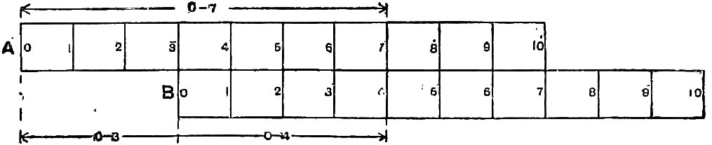

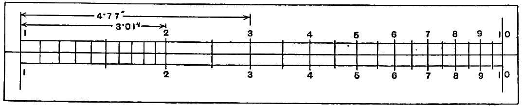


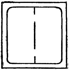
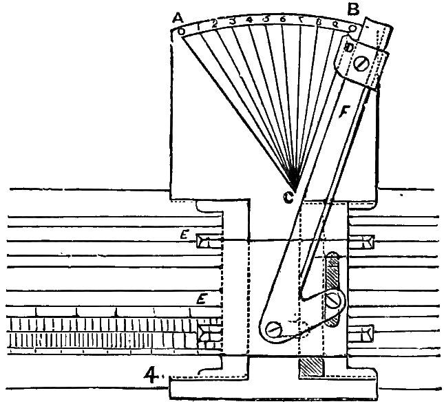
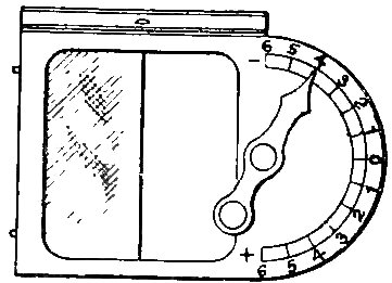
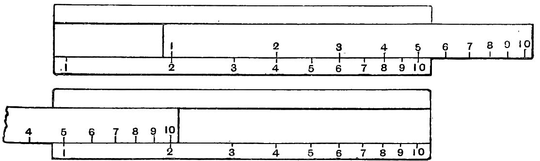
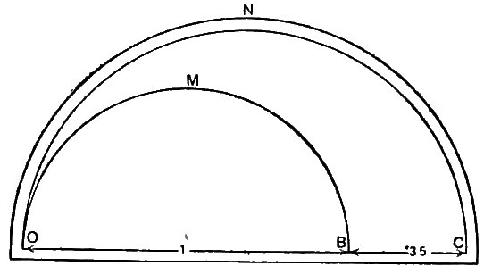
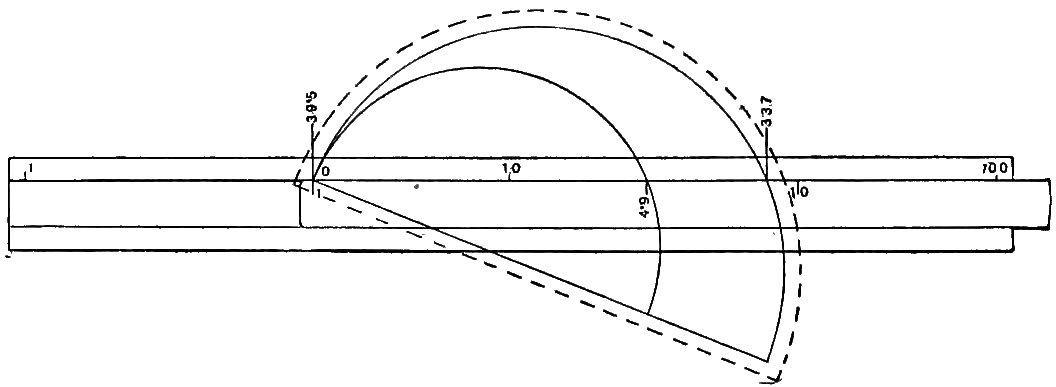
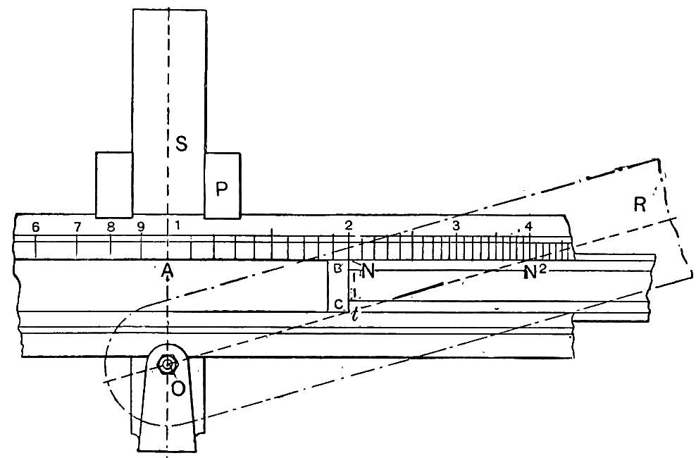
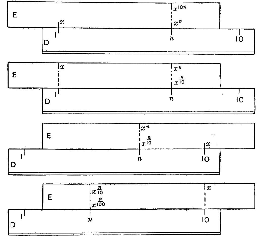
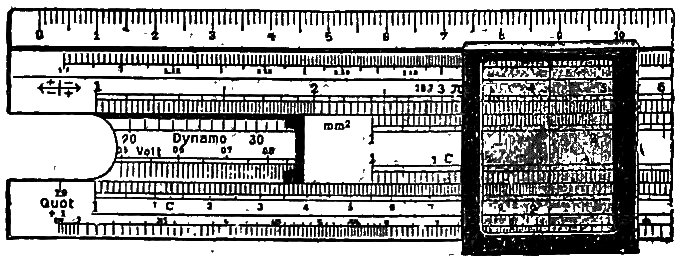
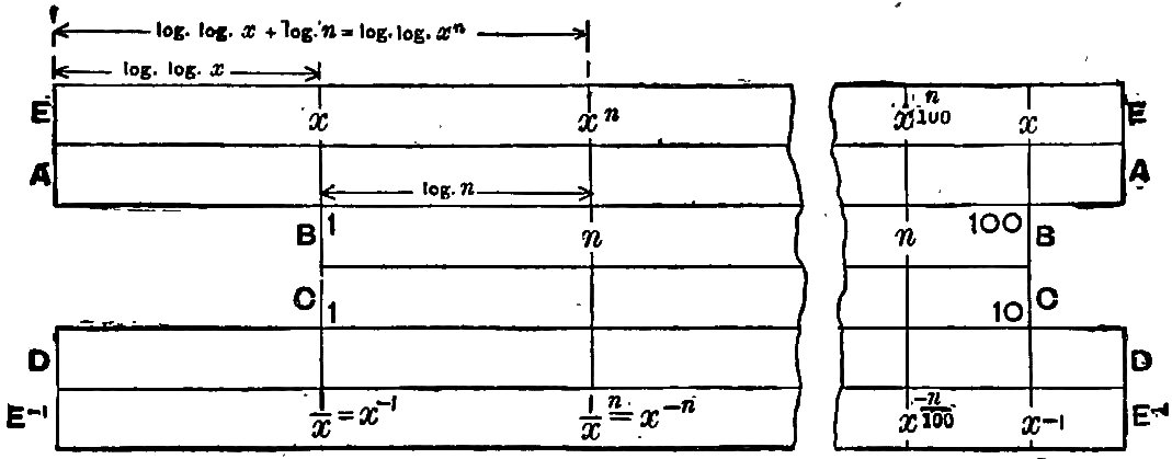

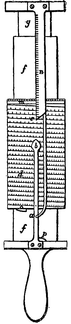

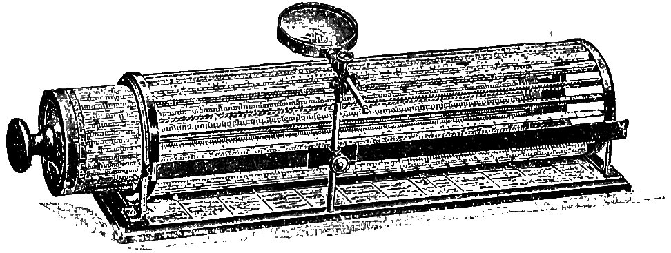
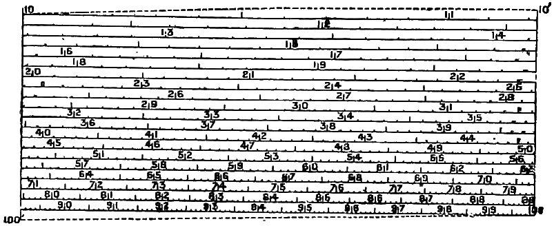
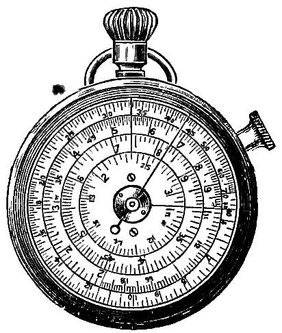
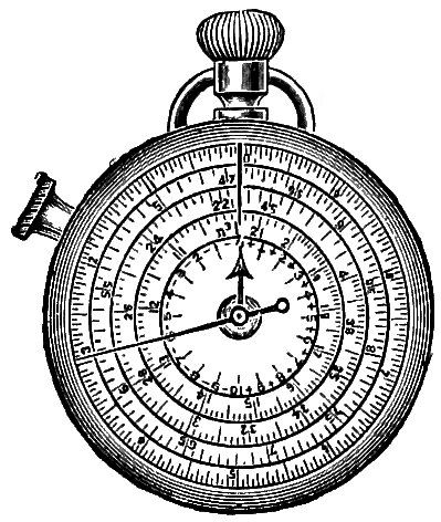
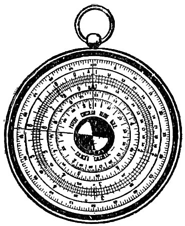
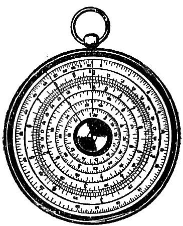
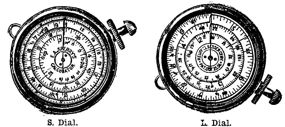
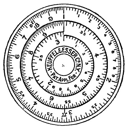
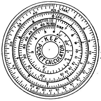
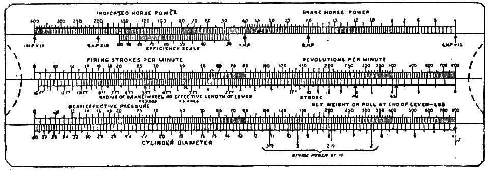
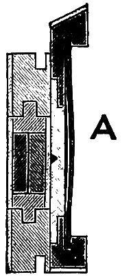
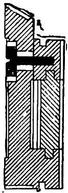
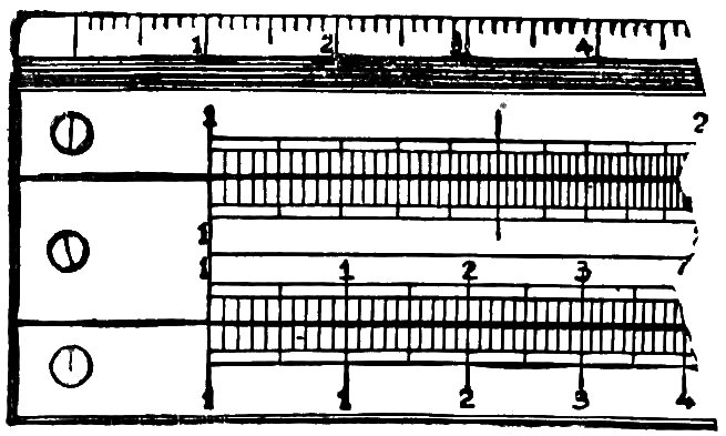

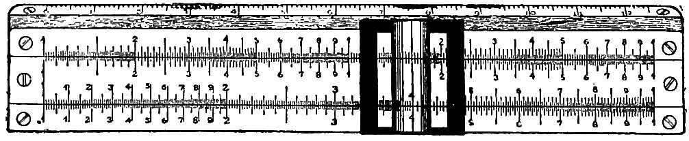

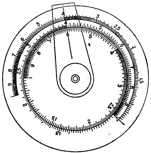
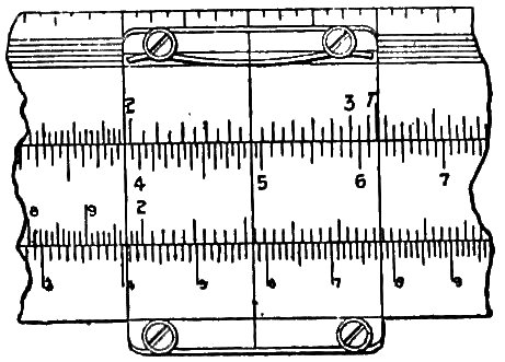

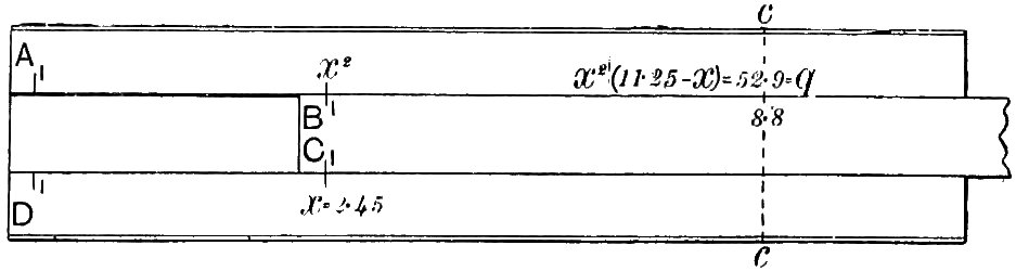
 found at both ends of the A scale is of general
application but of questionable utility. It is assumed to represent
a fraction, the vertical line indicating the position of the decimal
point. If the number 455 is to be dealt with in a multiplication
on the lower scales, we may suppose the decimal point moved
two places to the left, giving 4·55, a value which can be actually
found on the scale. If we use this value, then to the number of
digits in this result, as many must be added as the number of
places (two in this case) by which the decimal point was moved.
If the point is moved to the right, the number of places must
be subtracted. Similarly, in division, if the decimal point in the
divisor is moved n places to the left, then n places must be
subtracted at the end of the operation; while if the point is moved
through n places to the right, then n places must be added. The