49. Analytic Geometry. 49.1
Consider any time-system 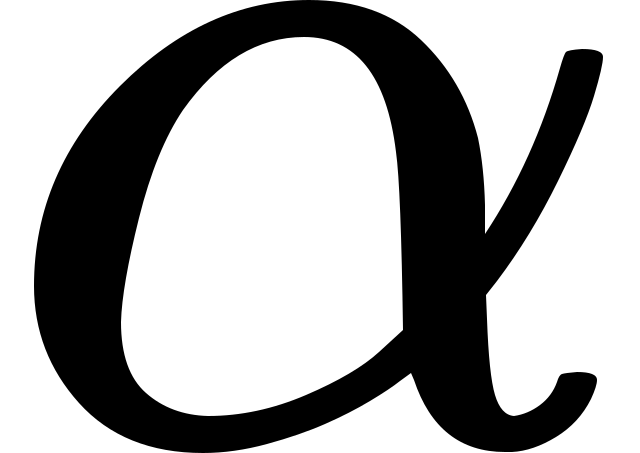 : we will term the space of this
time-system '-space' and its moments '-moments';
also the points and straight lines of -space will be termed
'-points' and '-lines,' and rects and levels which
lie in -moments will be termed '-rects' and
'-levels.' If
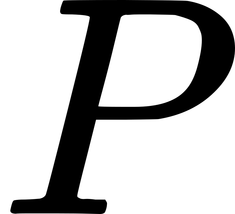 be any event-particle, then
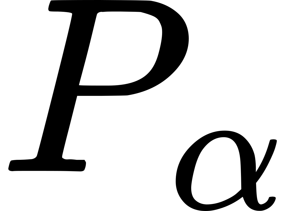 will denote the -moment which covers . If
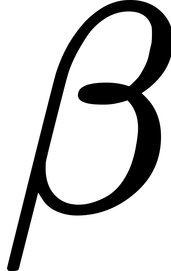 be
any other time-system, there are no -moments which are also
-moments, and no -points which are also
-points; but there are -levels which are also
-levels and -rects which are also -rects.
For the two moments and
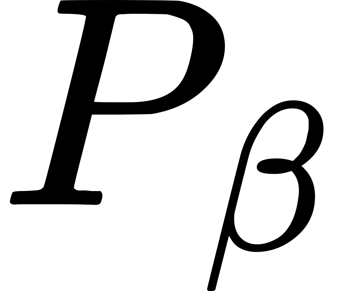 intersect in a
common level which will be called
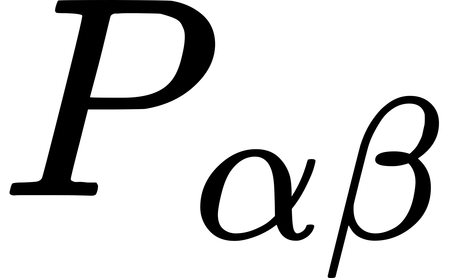 . Then rects lying
in are both -rects and -rects. In
particular through in the level pairs of
mutually normal rects exist, and every rect through and
is a member of one such pair.
49.2 Let 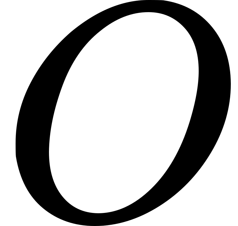 be any arbitrarily chosen event-particle, which we
will term the origin; and let
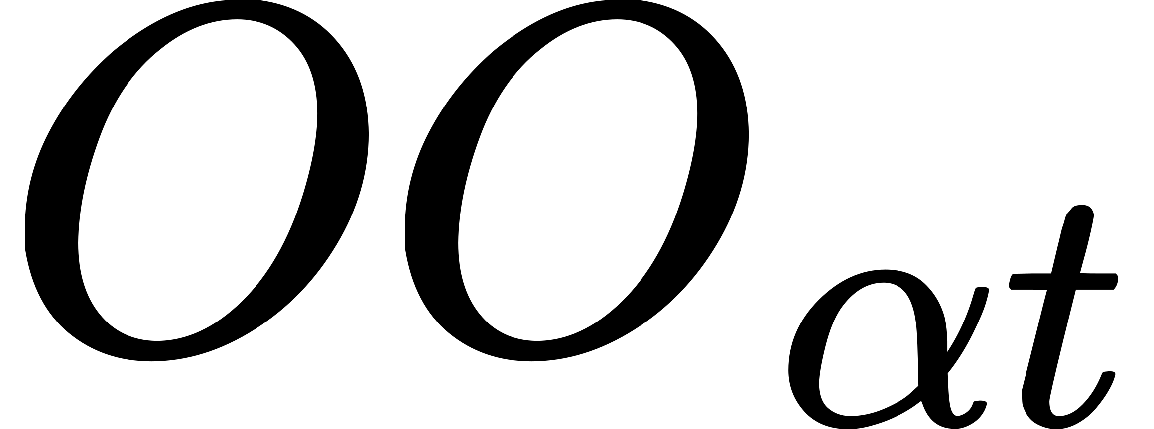 be the -point
occupied by ; and let
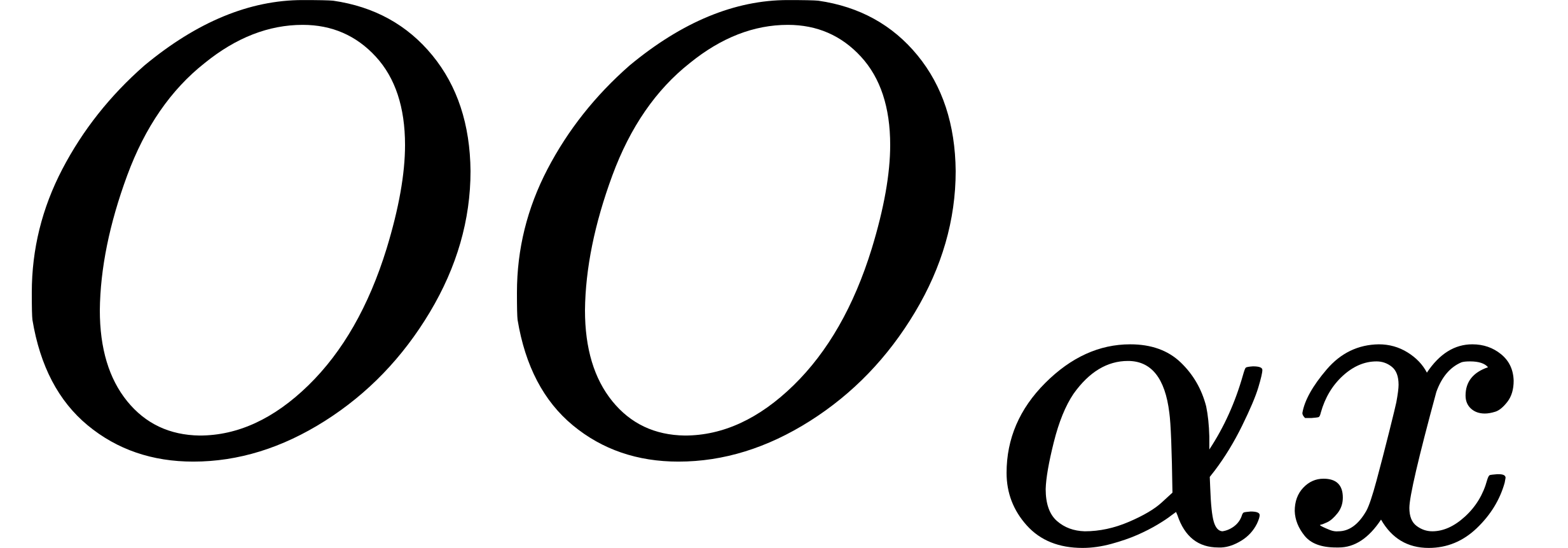 ,
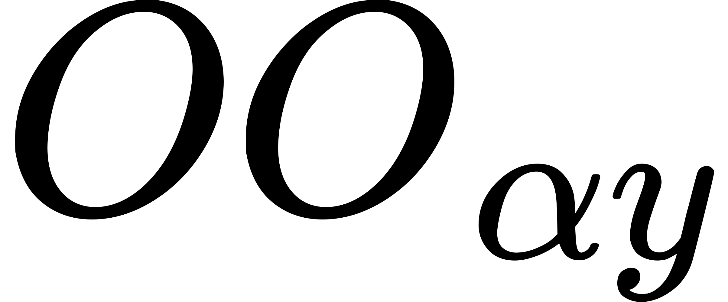 ,
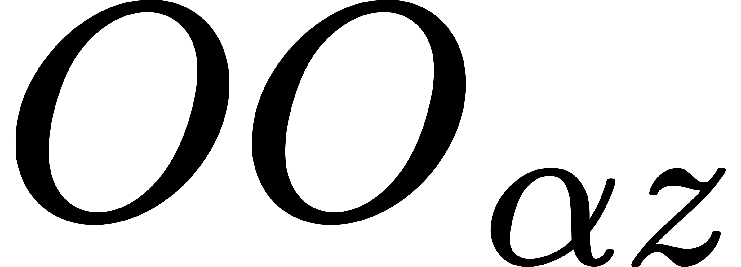 be any triad of mutually rectangular -rects
in the moment
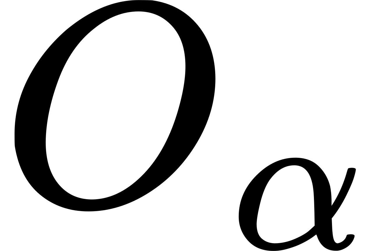 , each containing . In this notation
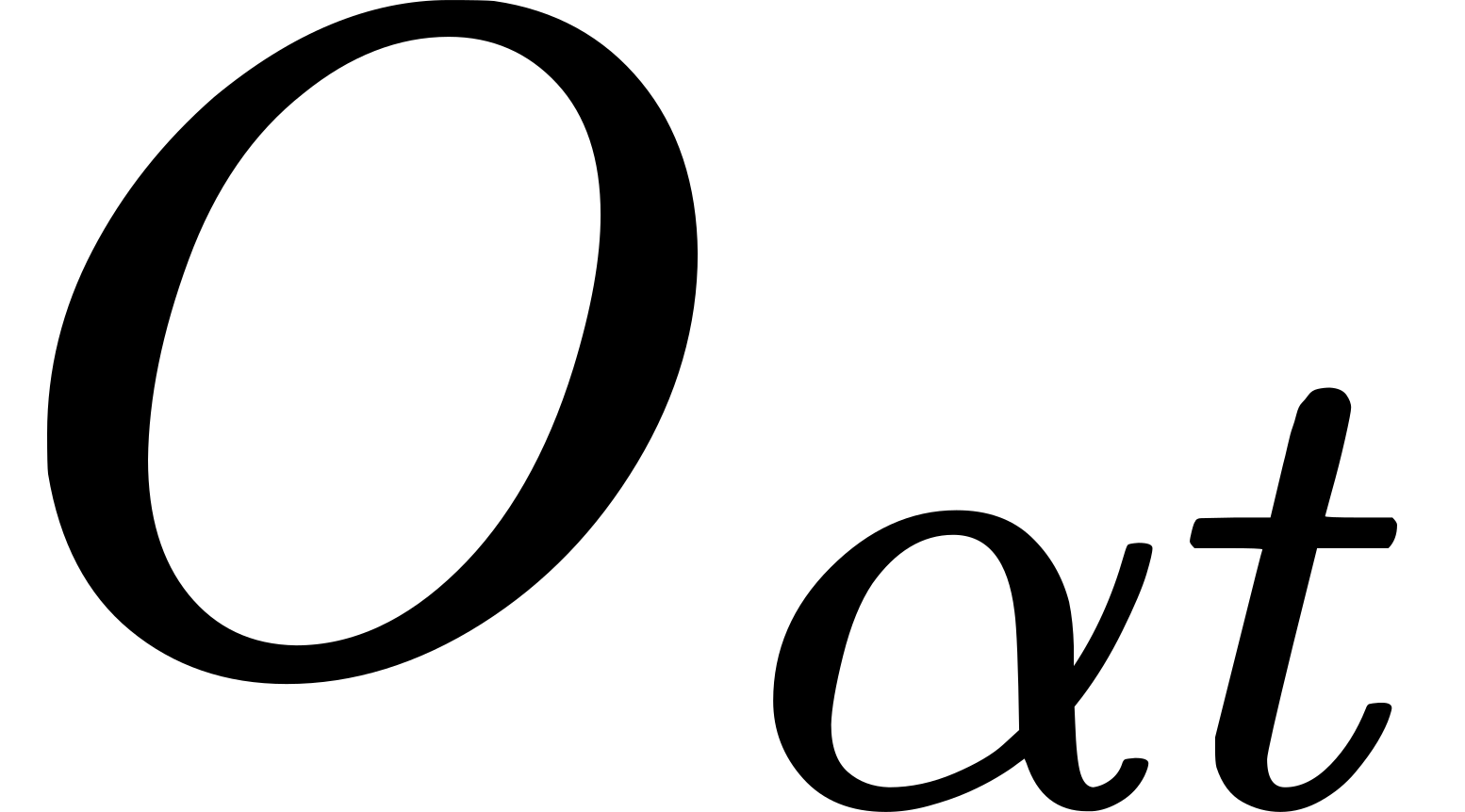 ,
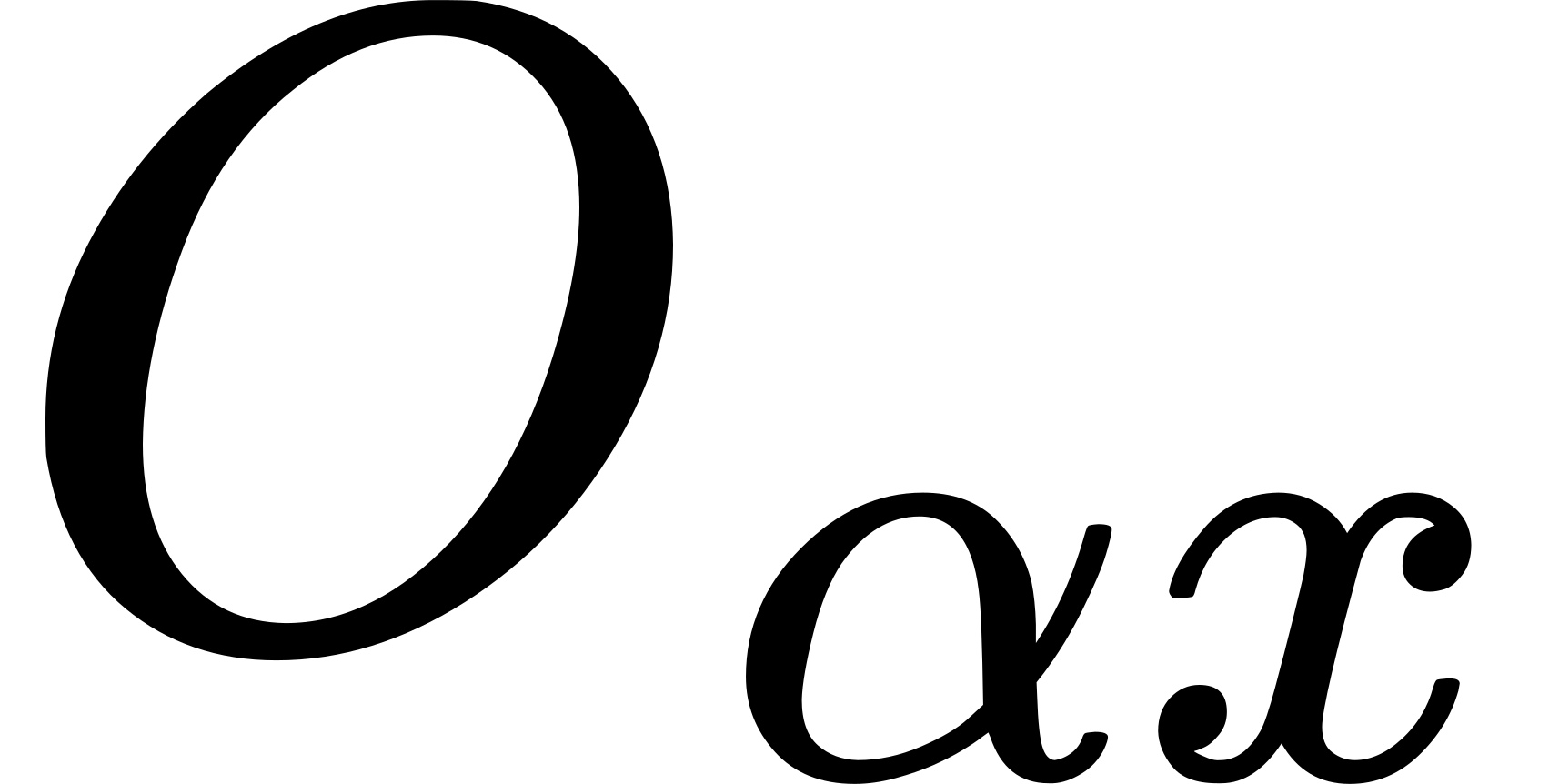 , etc., do not denote any particular
entities, but the symbols such as and
are each to be taken as one whole. Let
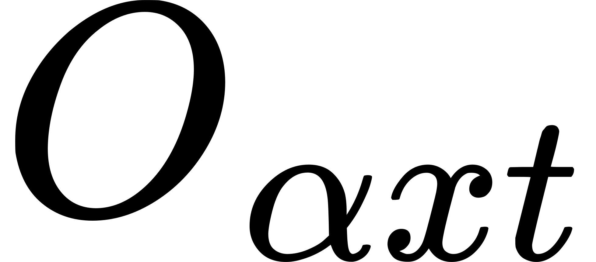 denote the
matrix containing and , with
analogous meanings for
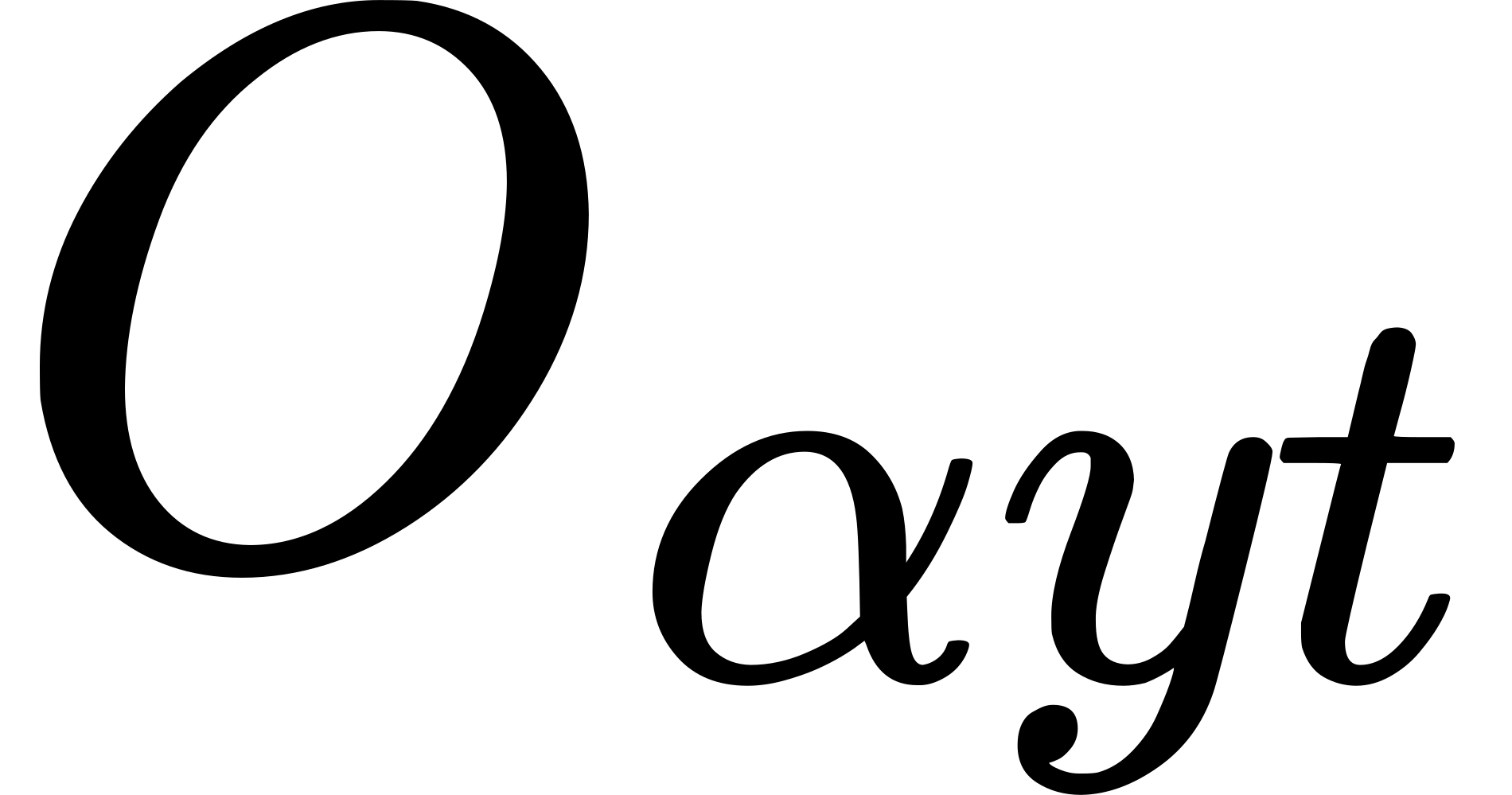 and
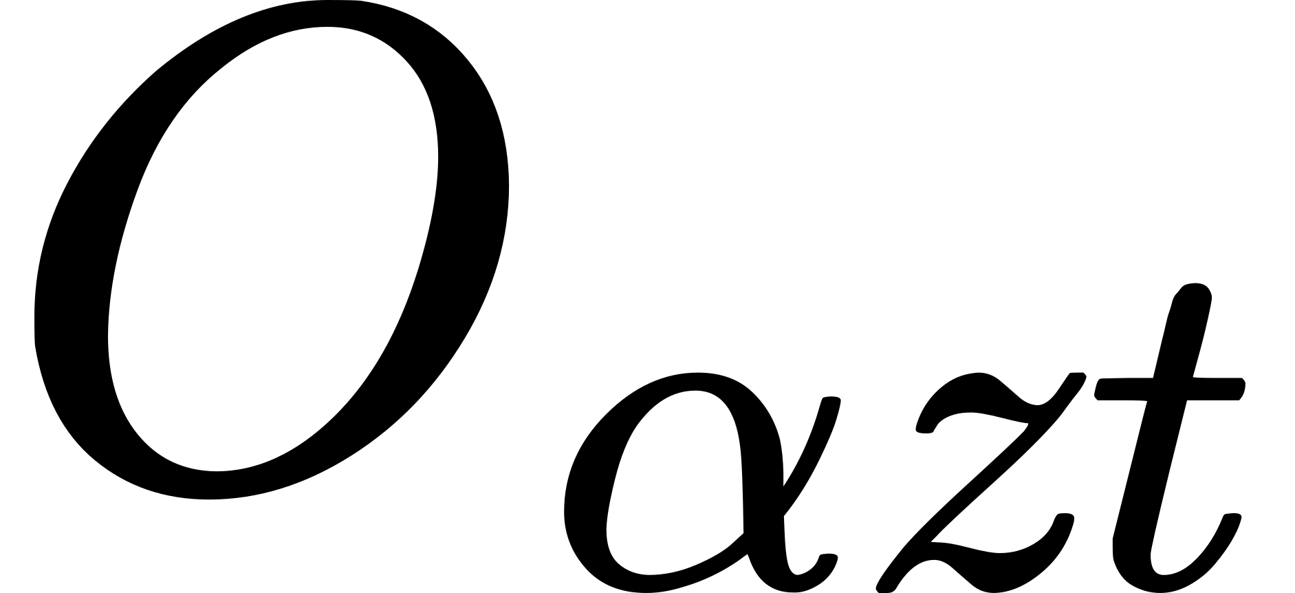 ; and let
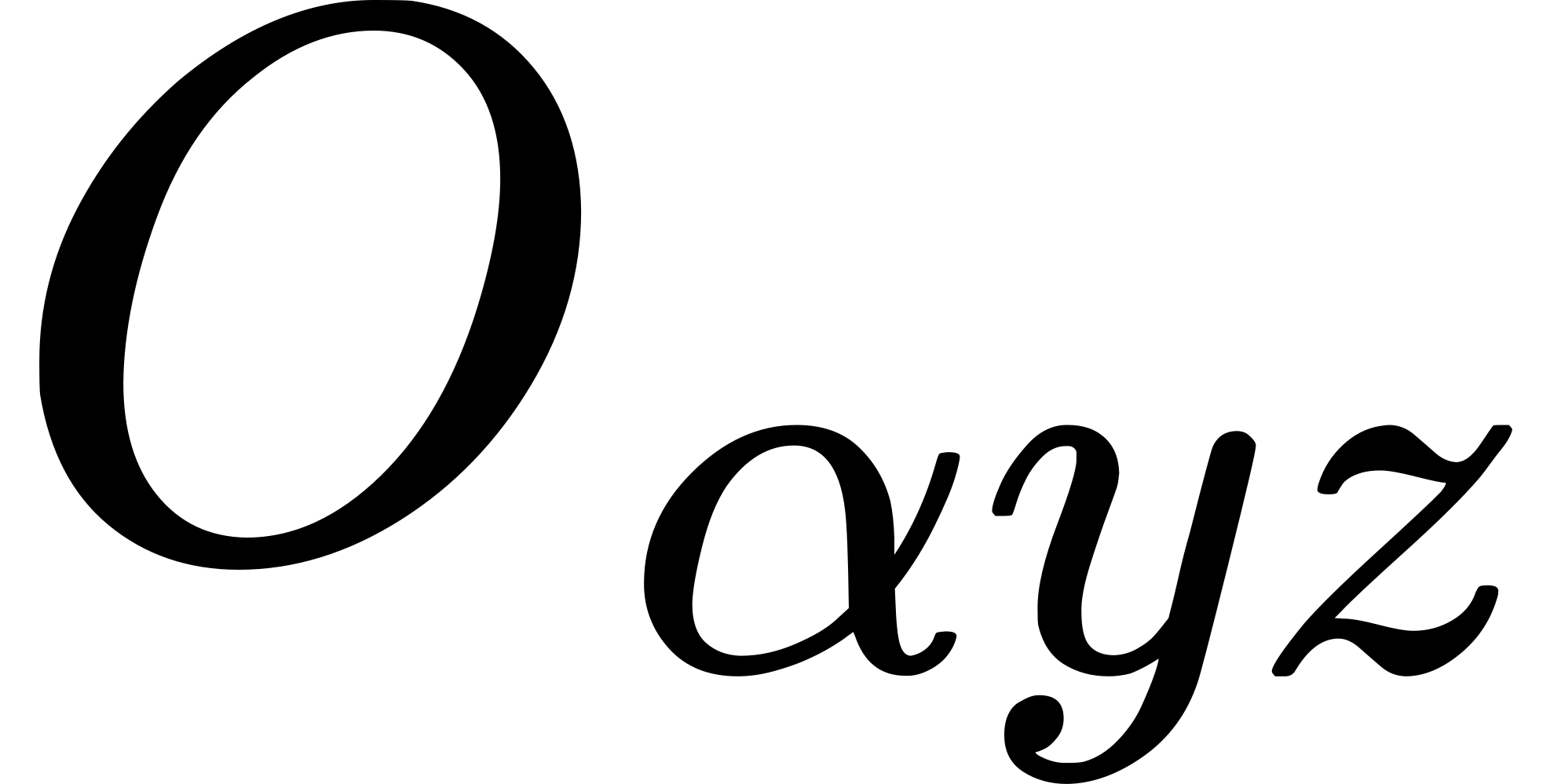 ,
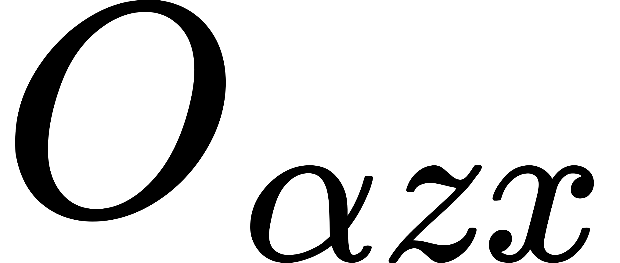 and
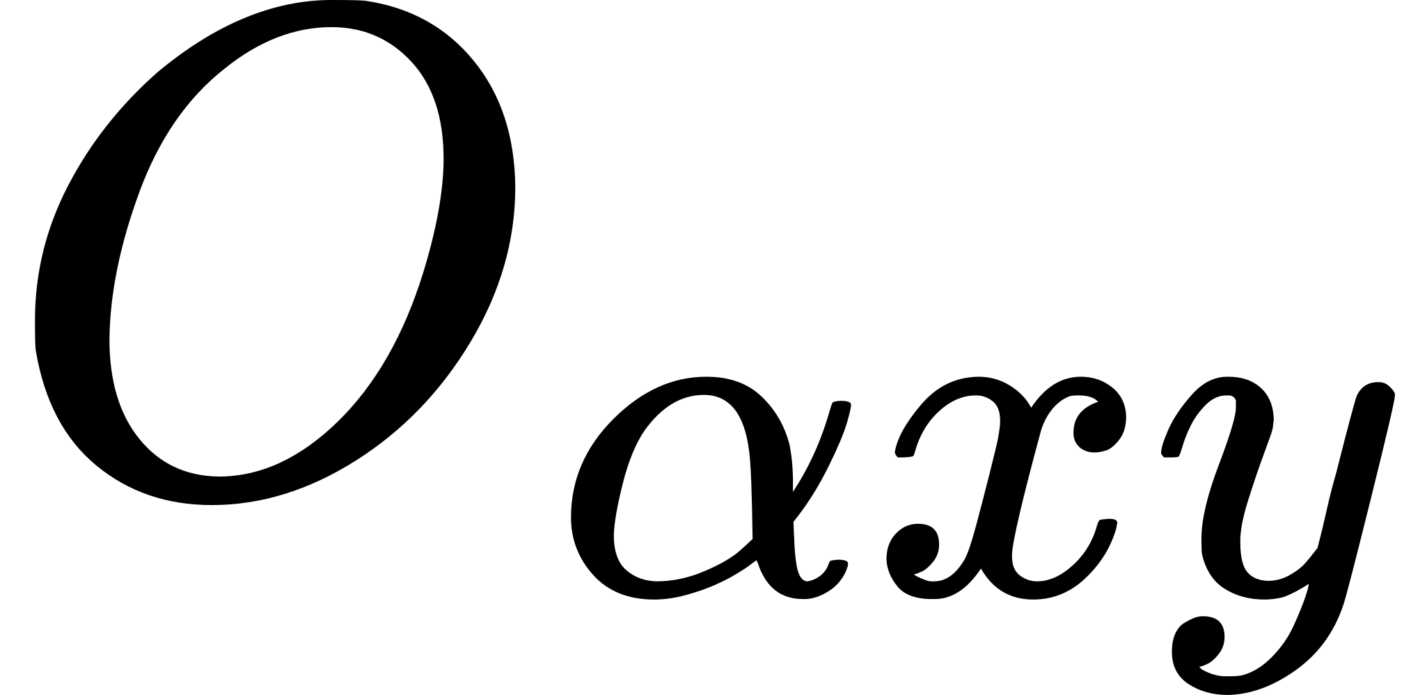 denote
respectively the levels containing and
, and
, and . Let be
any other event-particle occupying the point , and let
 be the
-rects through respectively parallel to
, , .
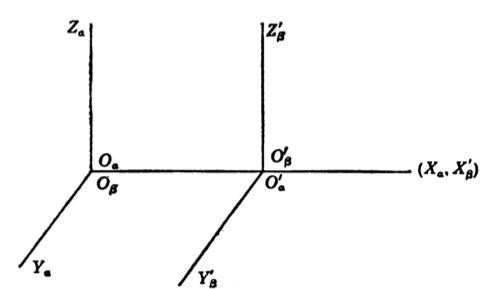
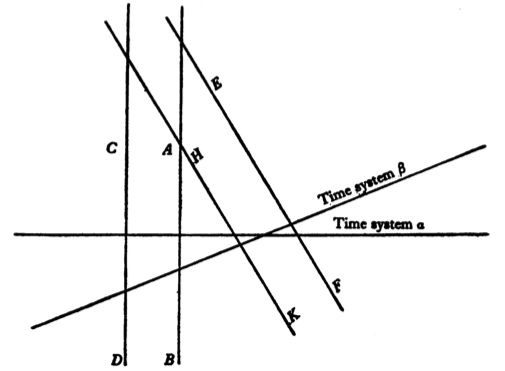
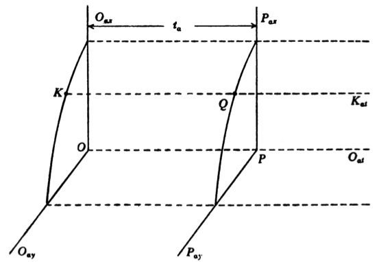
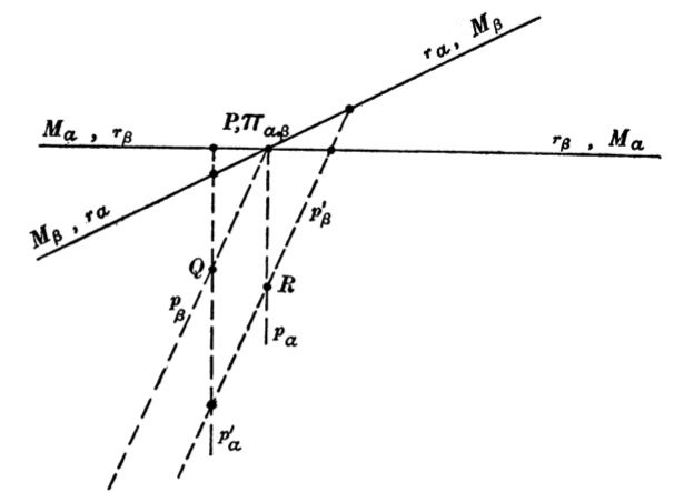
In the diagram the third dimension of the moments and
namely the 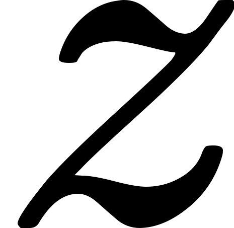 -dimension, is suppressed, so that these
moments are diagrammatically represented as two-dimensional.
Point-tracks (in this case -points) are represented by dotted
lines. The diagram has the defect of representing matrices, such as
, by levels, and is thus liable to lead to unfounded
assumptions.
49.3 Lengths on all rects, whether or no they be
-rects, are measurable in terms of one unit length. But
time-lapses between -moments—or, what is the same thing,
time-lapses along -points—must be measured in a
time-unit peculiar to the time-system , since as yet no means
of obtaining congruent time-units in different time-systems has been
disclosed. We will suppose at present that in each time-system there is
a given arbitrarily chosen unit for time-measurement.
49.4 Let the momentary space of be referred to the
three rectangular -rects , ,
as axes of coordinates; and let the momentary space of
be referred to the three rectangular -rects
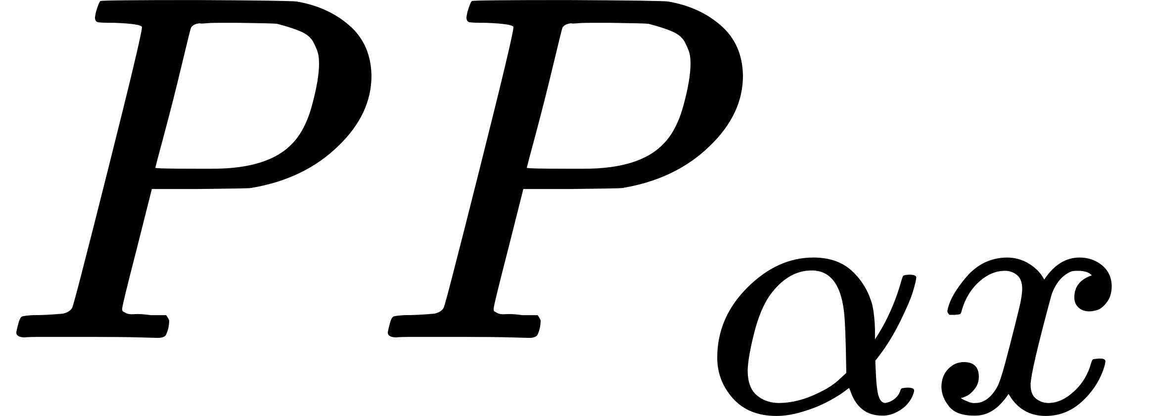 ,
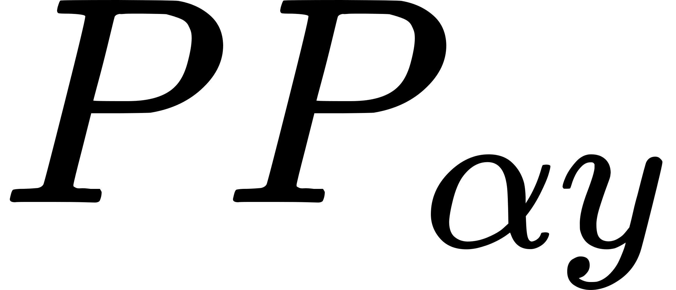 ,
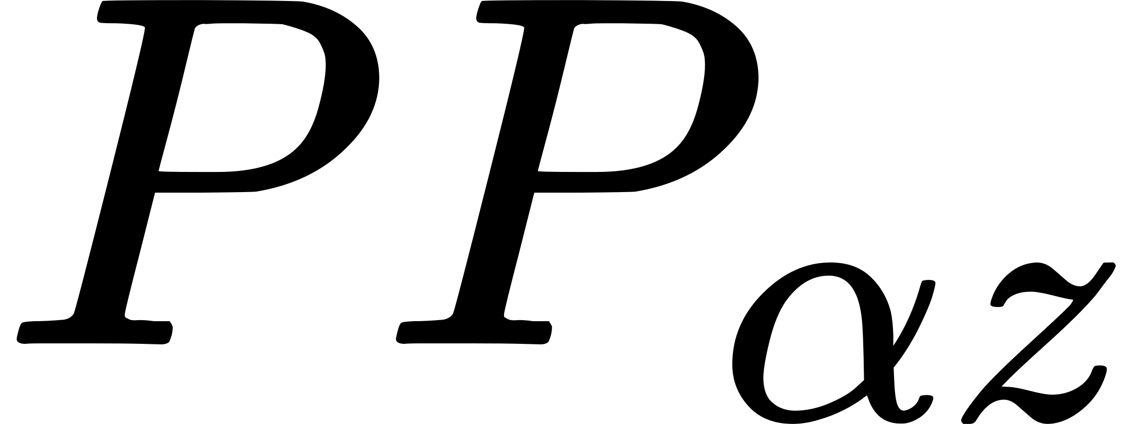 as axes of
coordinates; and let the time-less space of a [the -space] be
referred to the three rectangular -lines respectively included
in the matrices , ,
as axes of coordinates; and let the four-dimensional space of all
particles be referred to the four axes consisting of the three
-rects , , ,
and of the -point as axes of co-ordinates.
49.5 Let 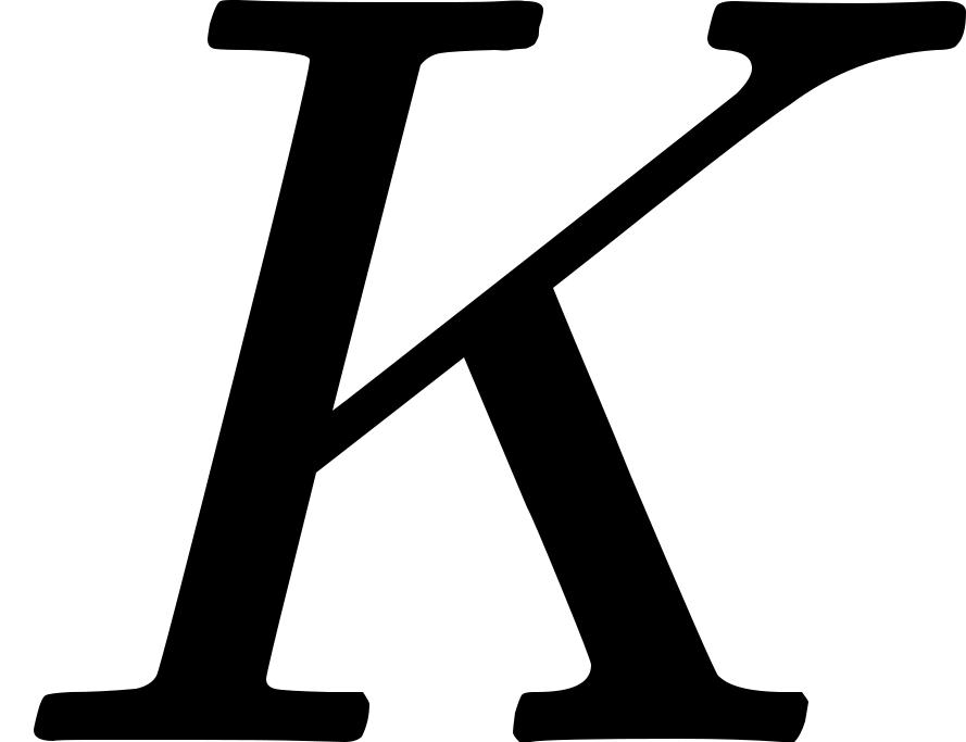 be any event-particle in the moment
, and let occupy the -point
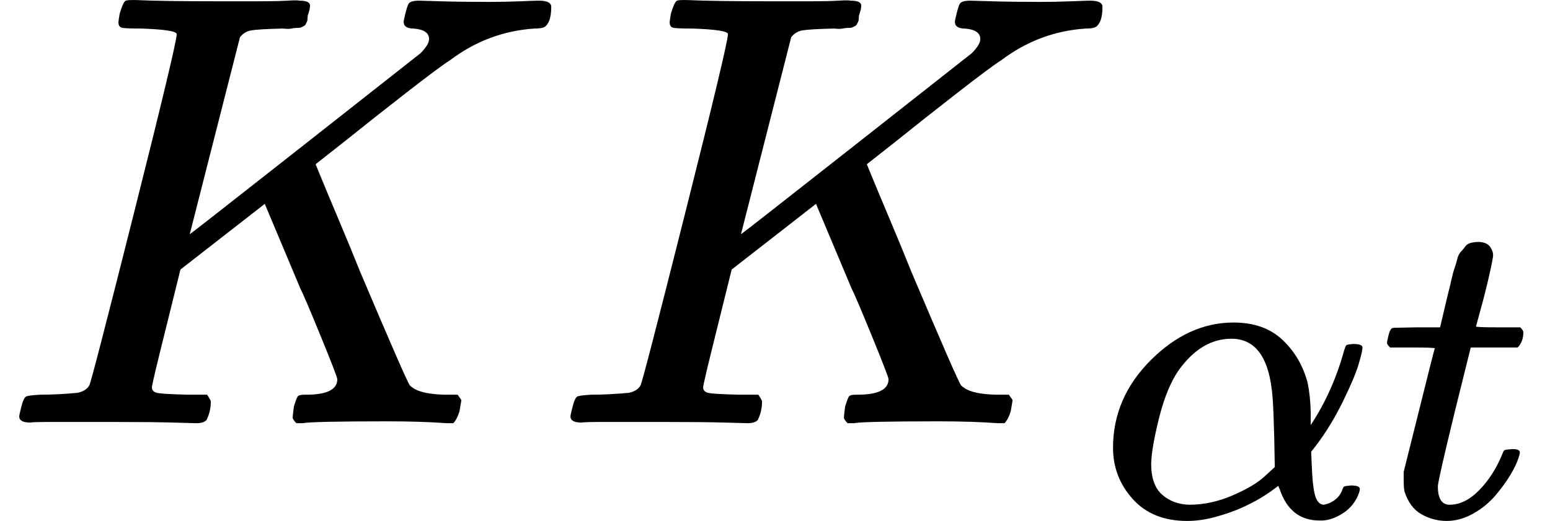 which intersects the moment in the event-particle
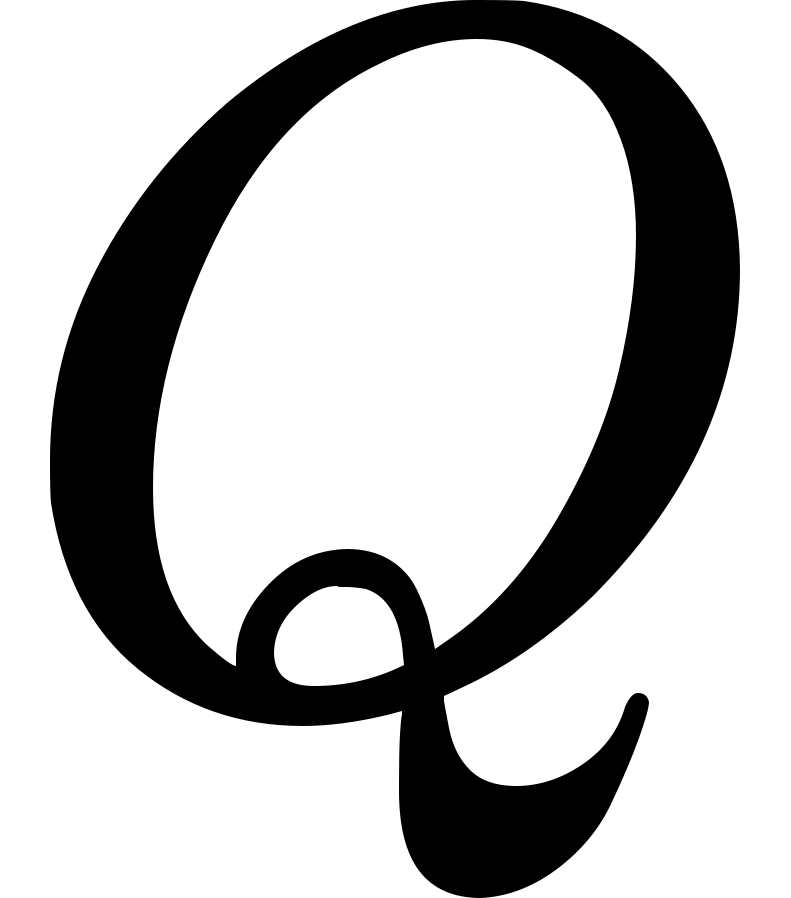 . Let the lapse of time between the moments and
be
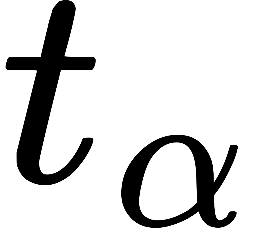 , where is positive when
is subsequent to ; and let the coordinates
of the -point in the -space be
(
 ). Then the coordinates of
in the momentary space of and of in the momentary
space of are also
(). Also the '-coordinates'
of in the four-dimensional space of particles are
(
 ); this fact for
can also be expressed by saying that occupies the
-point ()
at the -time .
A moment, viewed as a locus of event-particles, is represented
by a linear equation in the four coordinates
().
But the converse is not true; namely, not every linear equation
represents a moment. A pair of linear equations represent a level or
a matrix, and three independent linear equations represent a rect or a
point-track or a null-track.
49.6 If and be any two time-systems, two
sets of mutually normal axes,
 ,
and
 ,
can be found as in the previous subarticle. But these
two sets can evidently be so adjusted that is
identical with
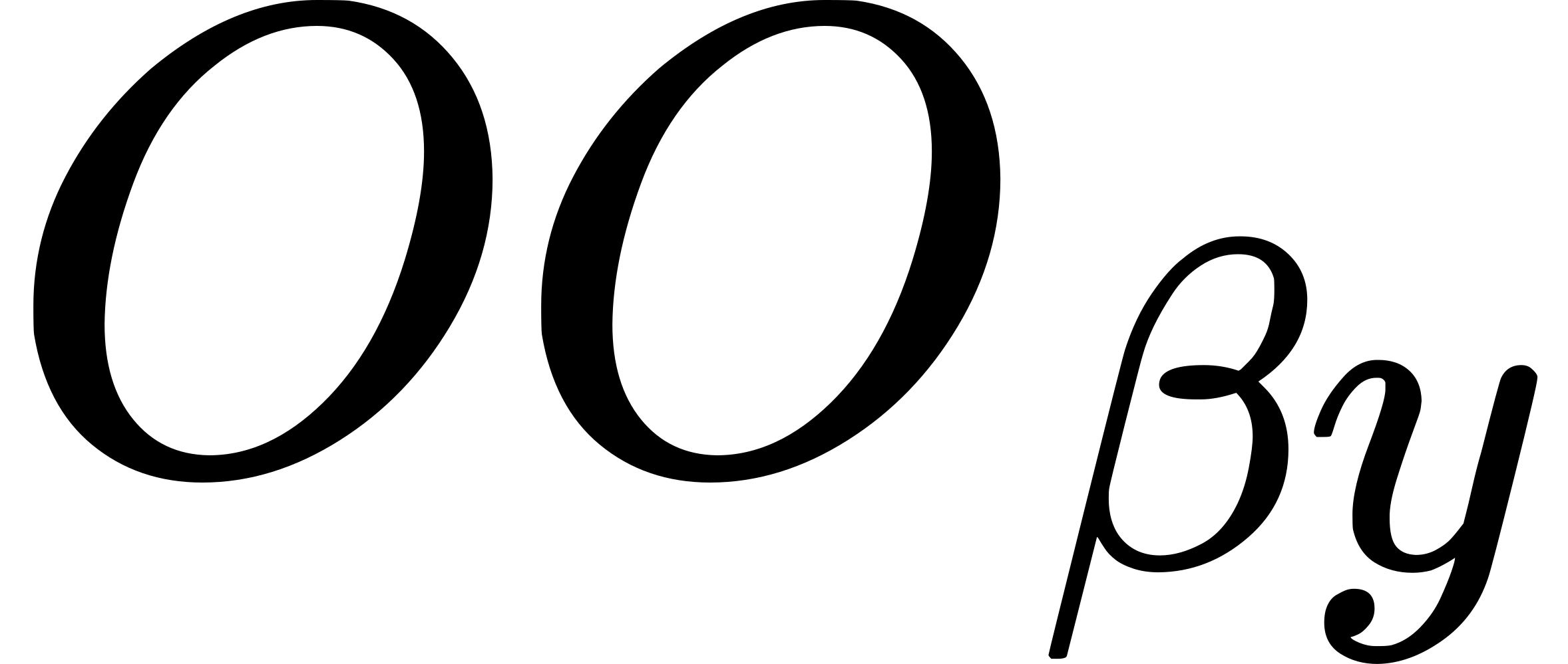 and is identical with
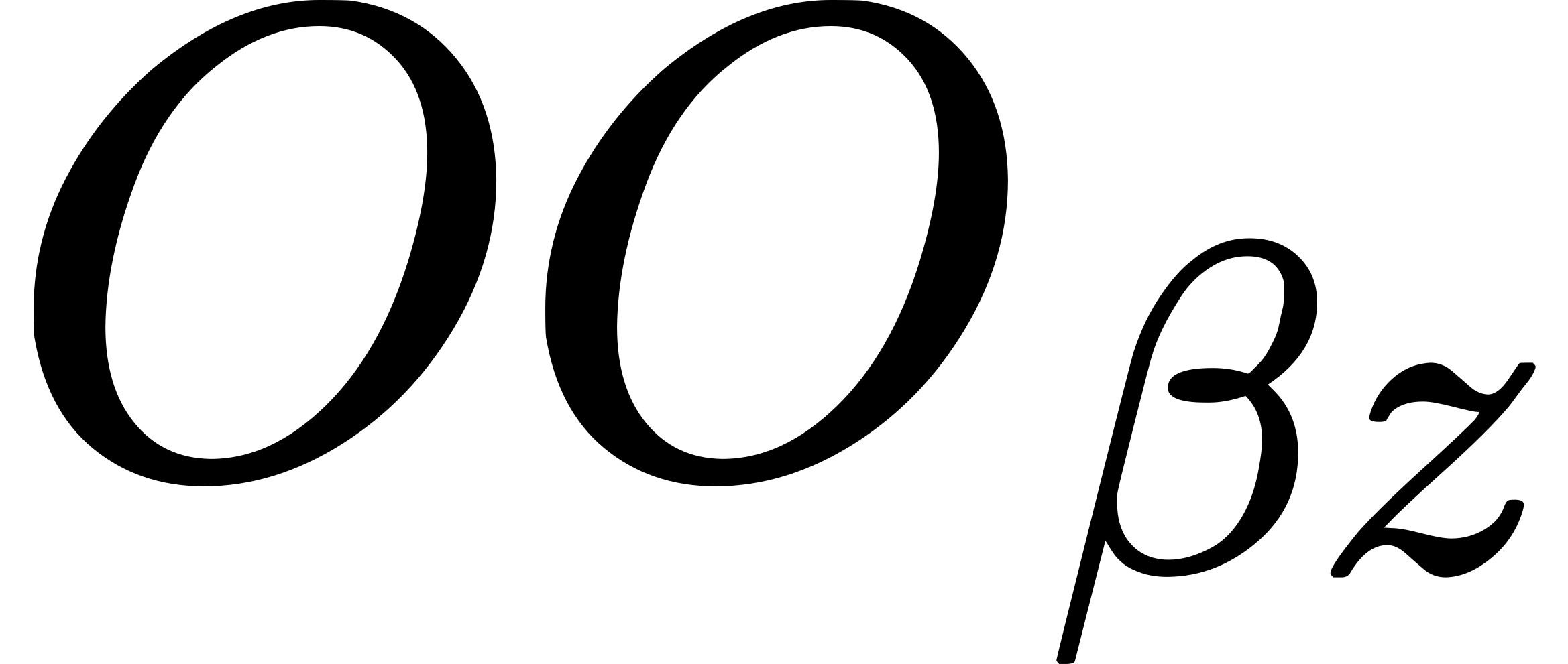 , where the two rects
(
 ) must both lie in the
level
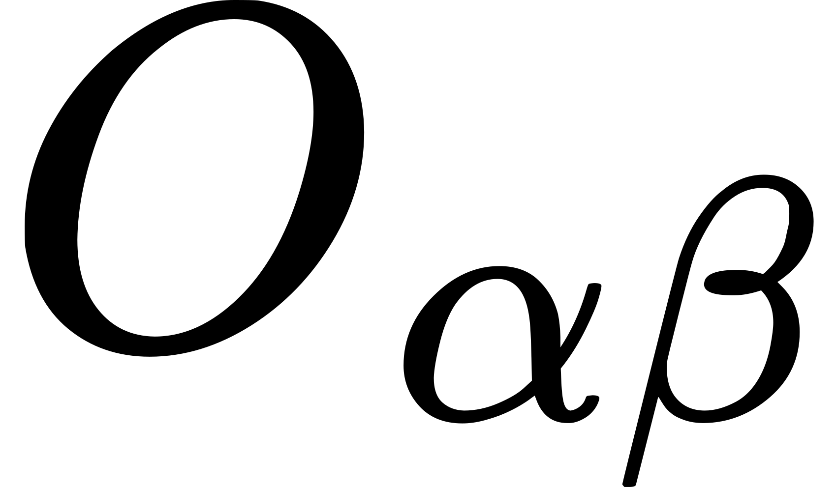 .
Then the matrix normal to this level at will be denoted by
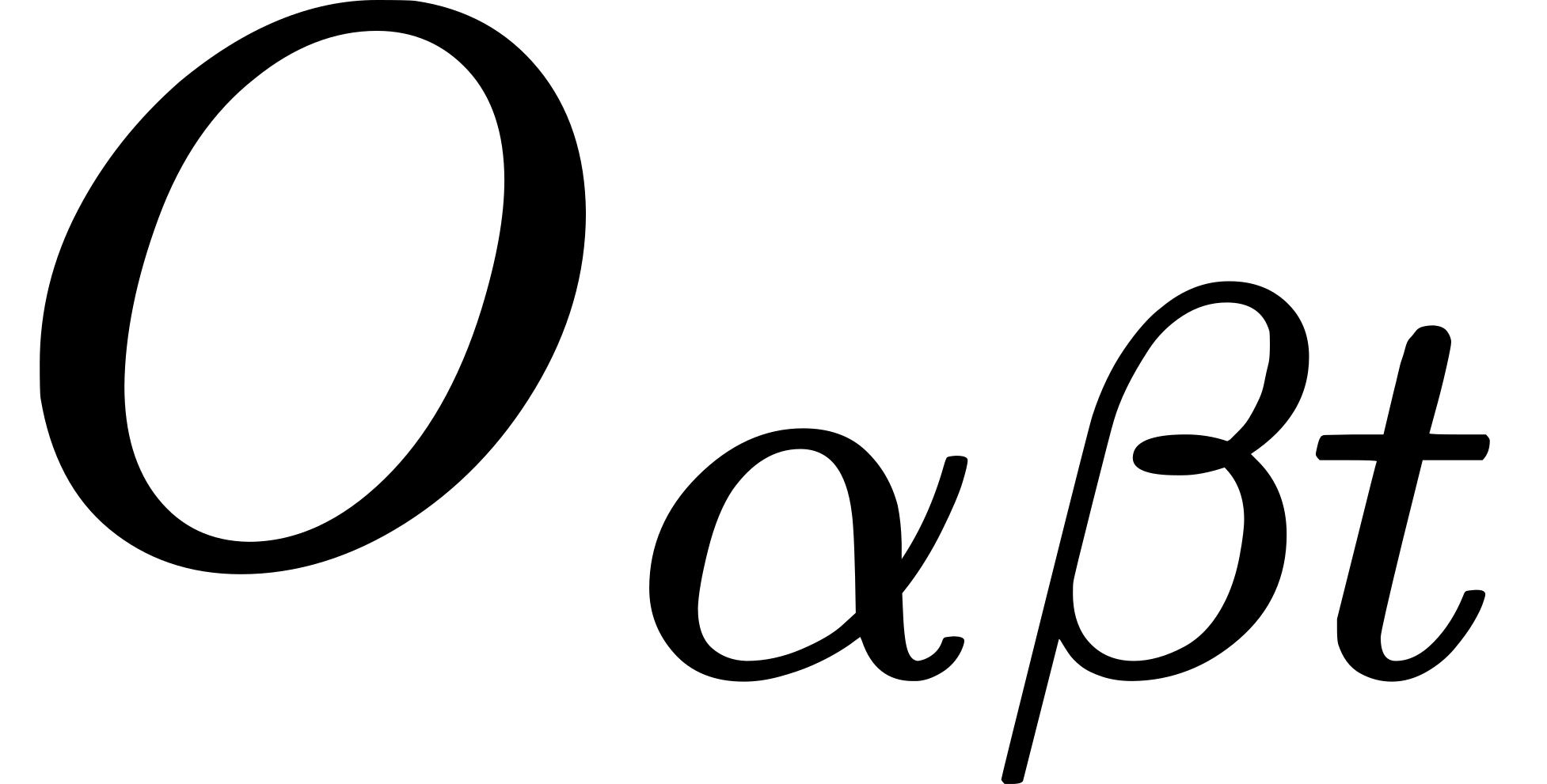 ; it contains through one -point
, one -point
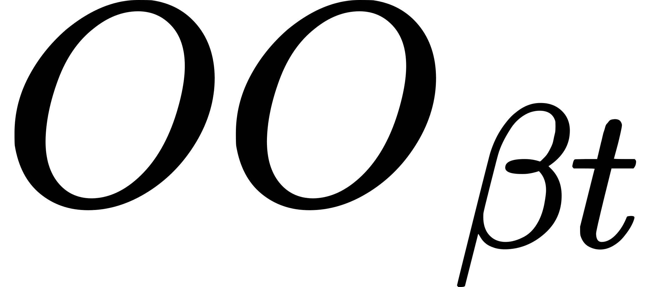 one
-rect , and one
-rect
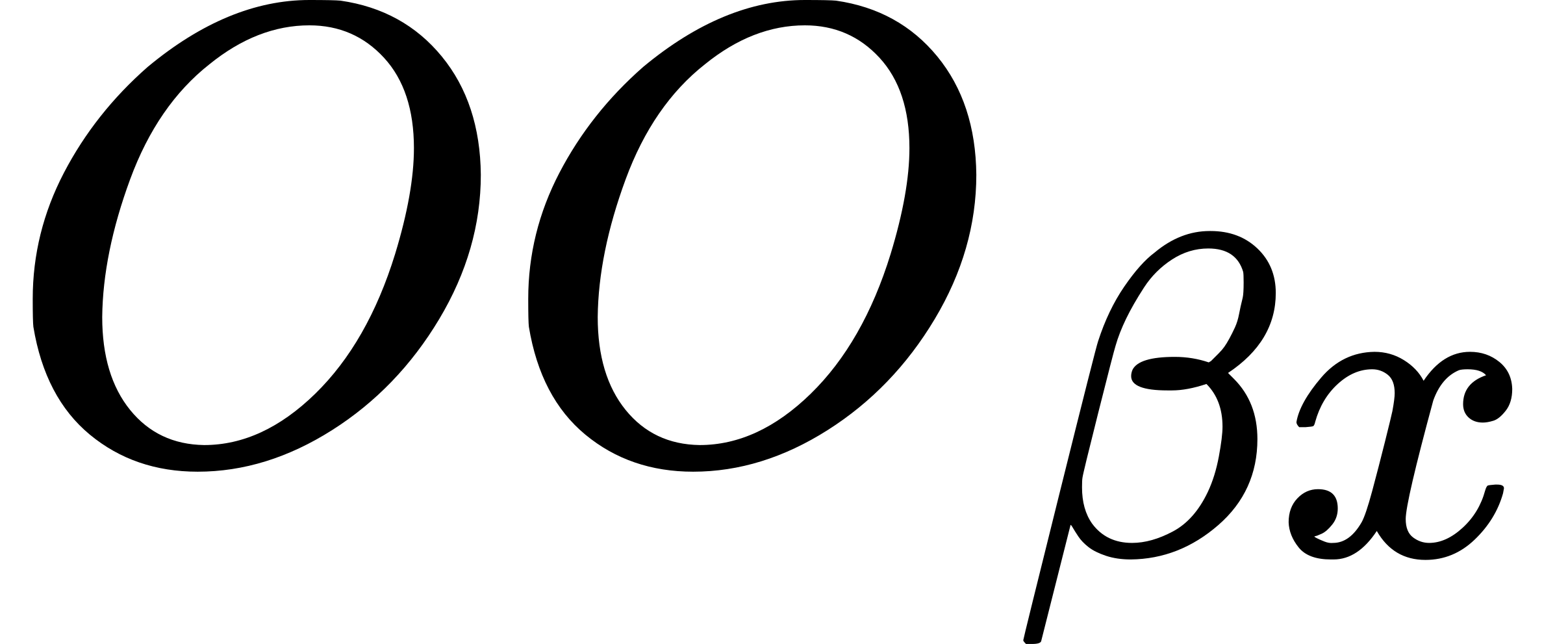 . Then any event-particle is referred
to the axes
for the system , and to the axes
for the system . Let its -coordinates be
() and its
-coordinates be (
 ),
where
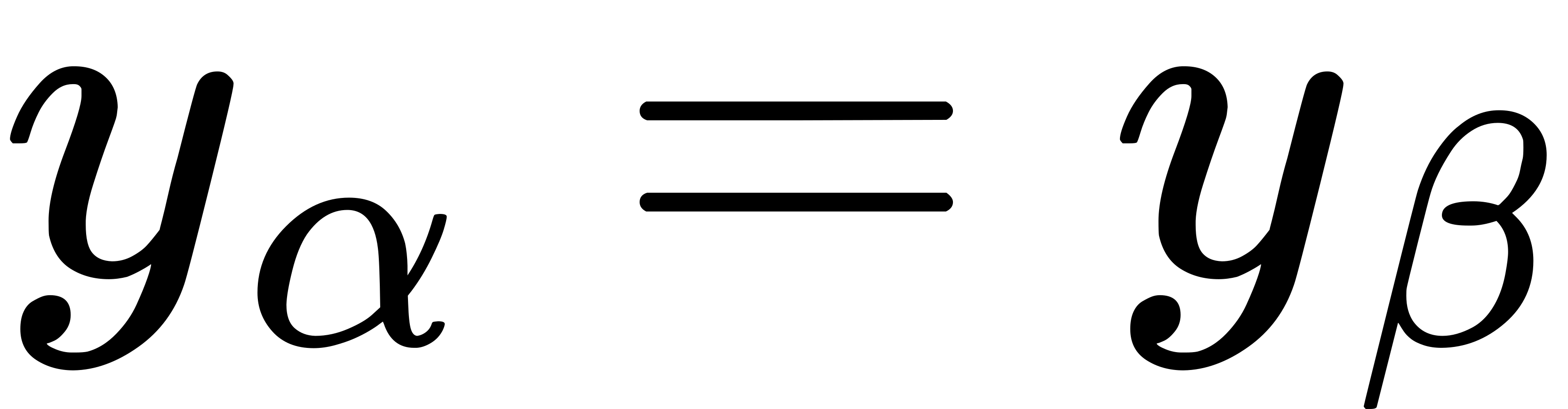 , and
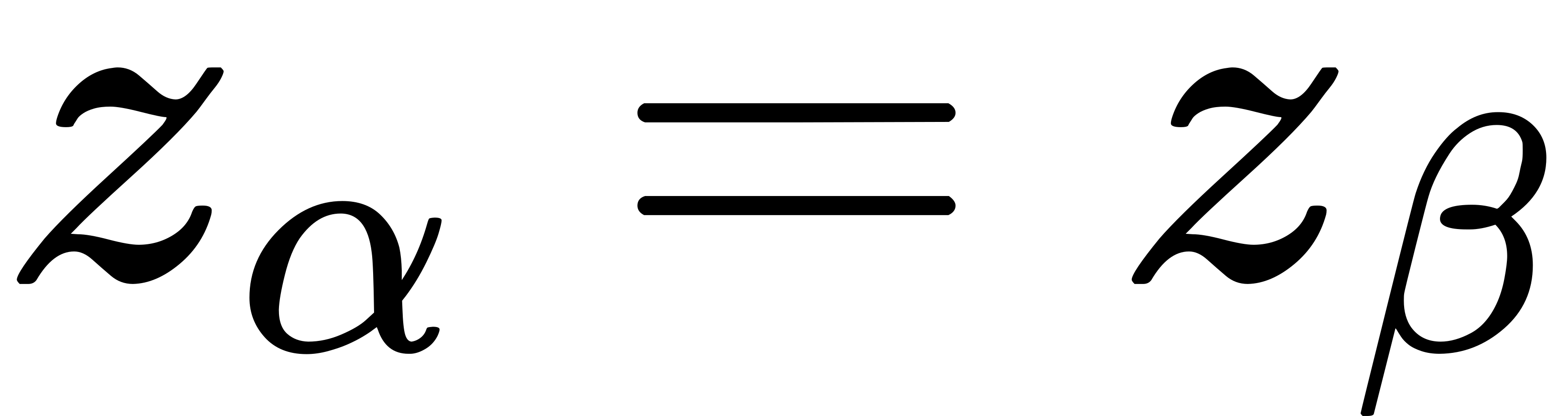 .
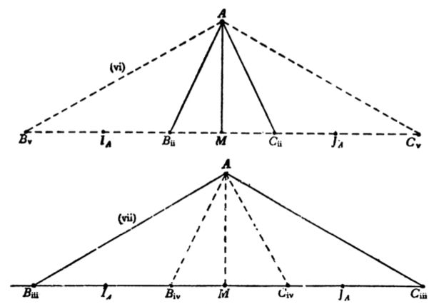
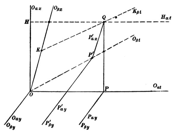
In the diagram, for the sake of simplicity, the particle
is in the matrix ; and its coordinates [as in the
diagram] in the two systems are ( )
and (
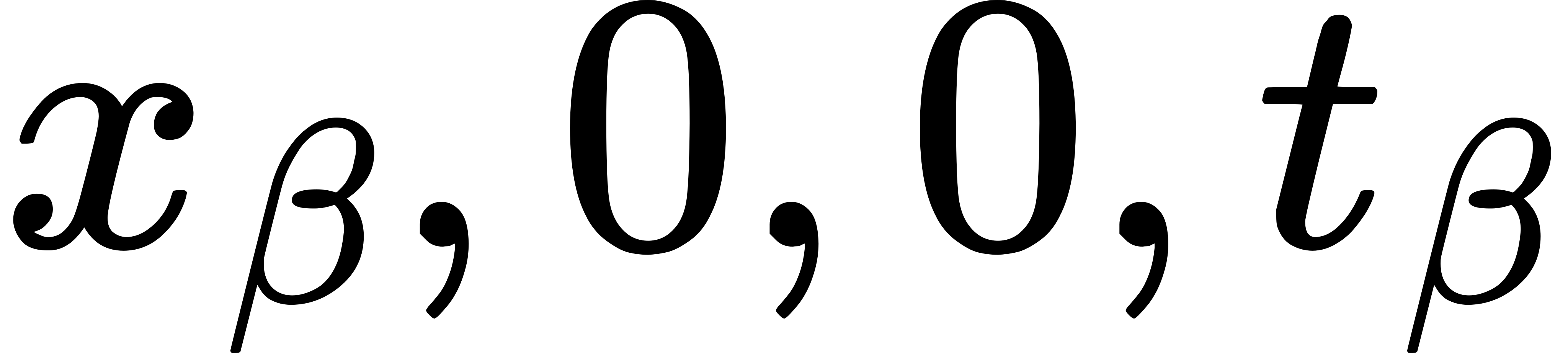 ), where
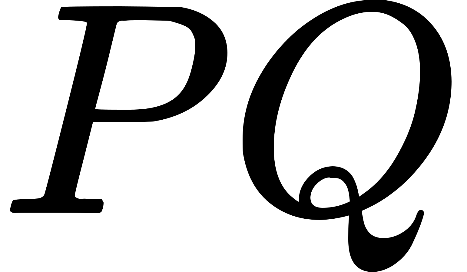 (with its proper sign) is
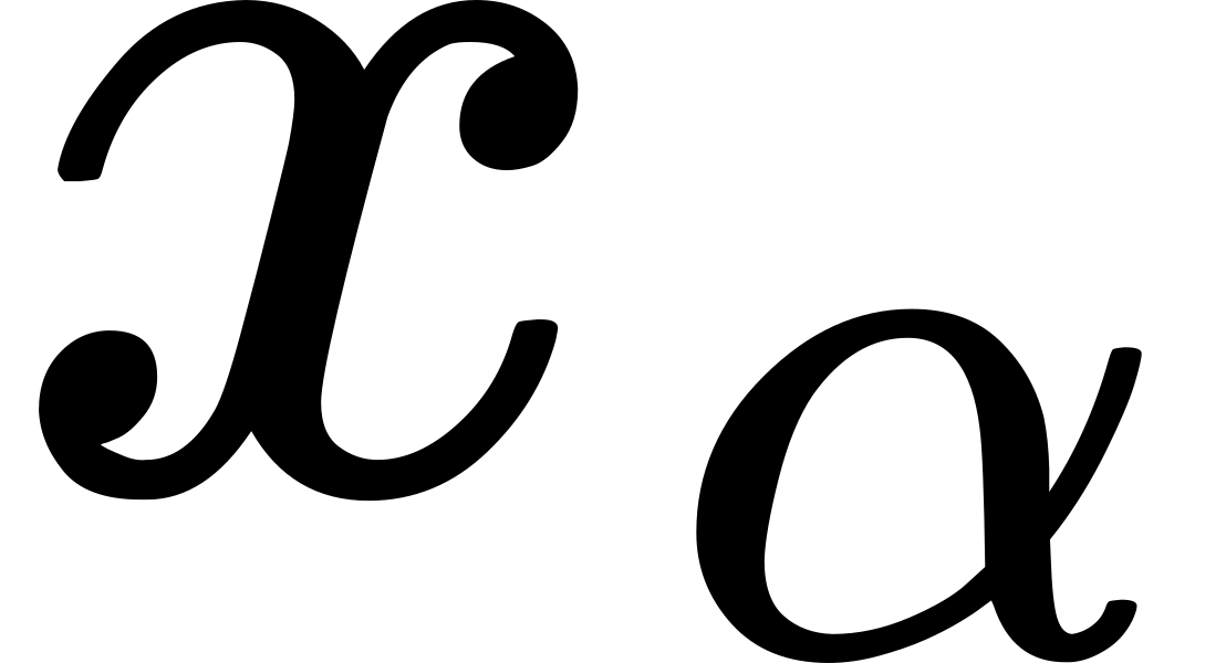 ,
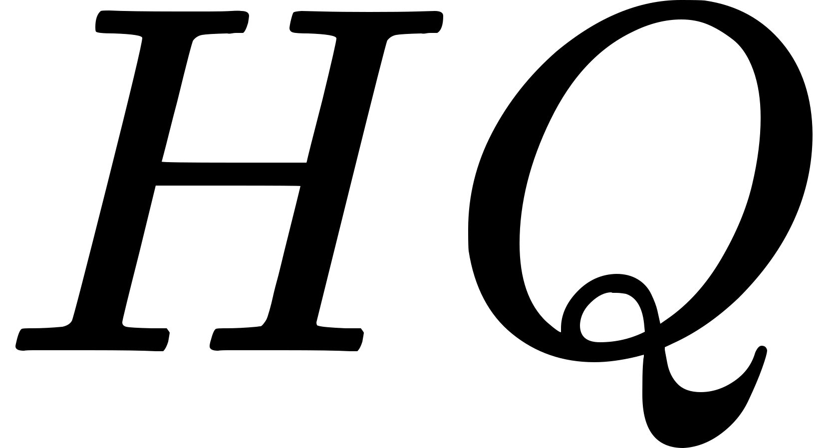 (with its proper sign) is ,
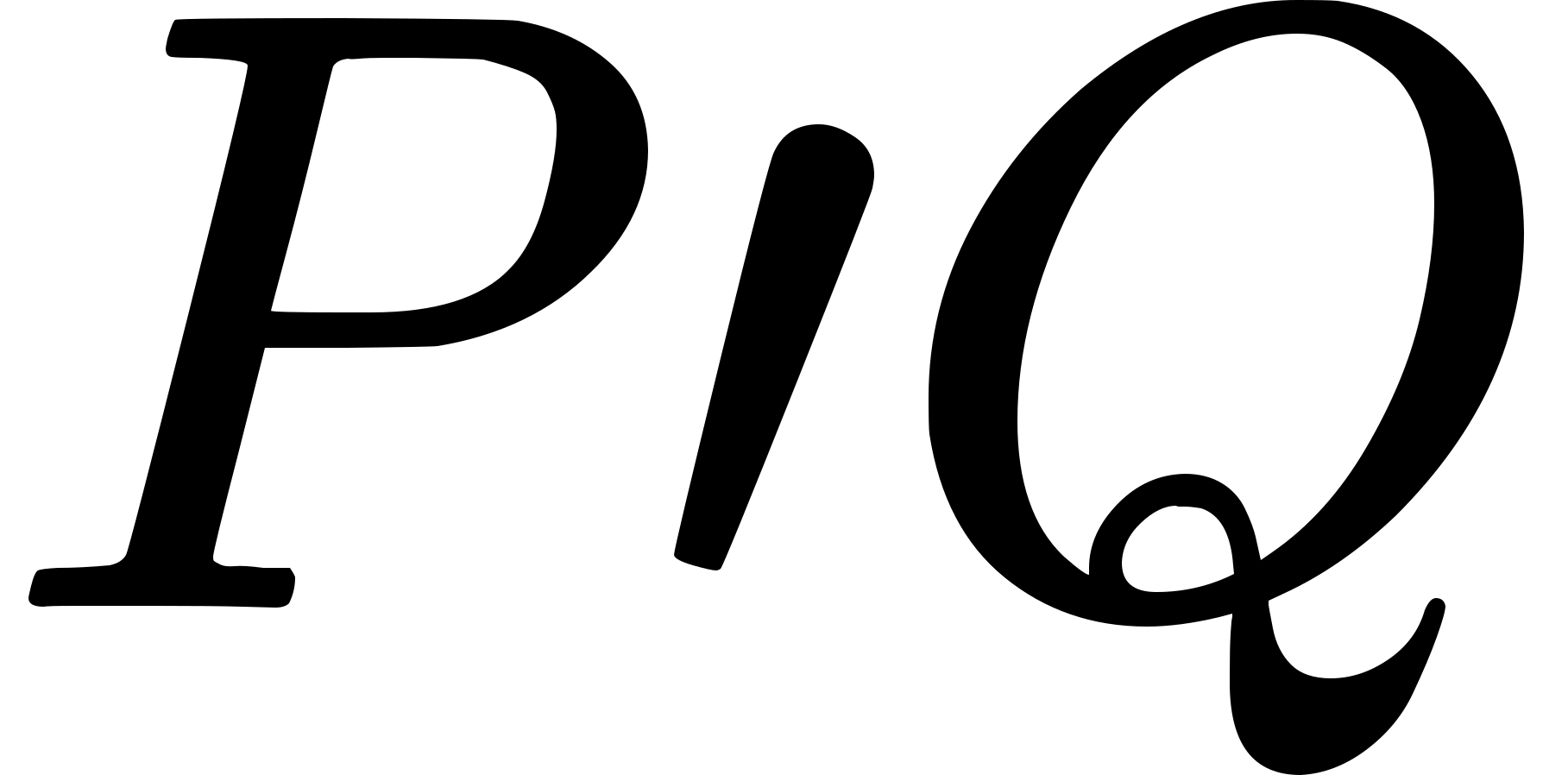 (with its proper sign)
is
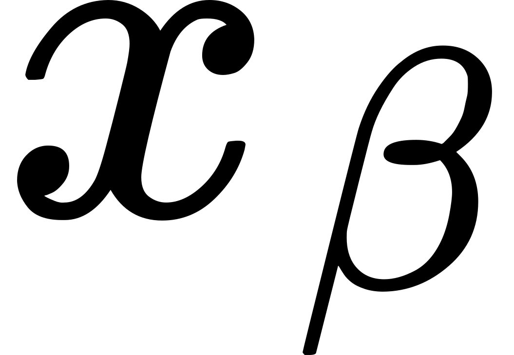 , and
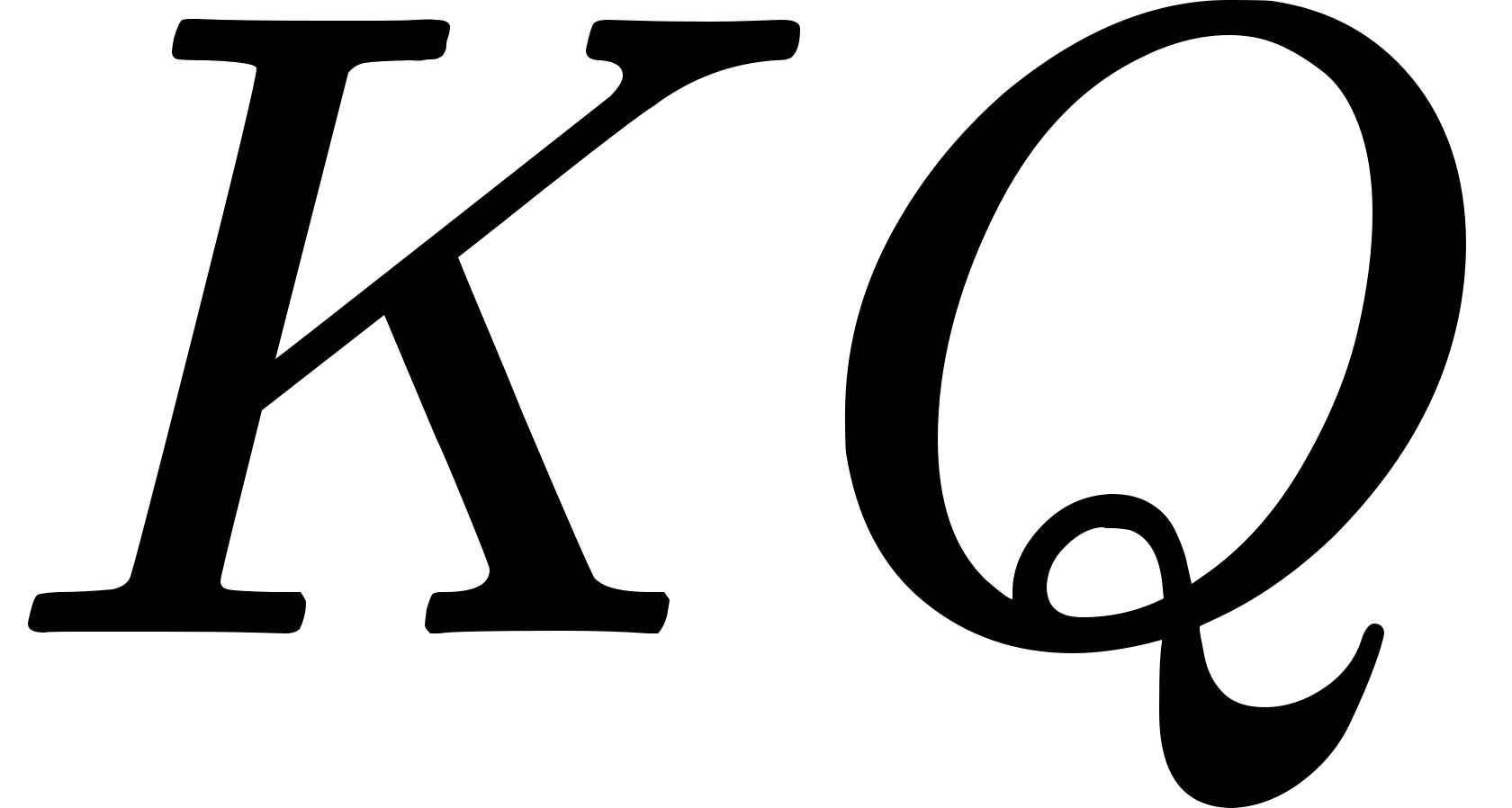 (with its proper sign) is
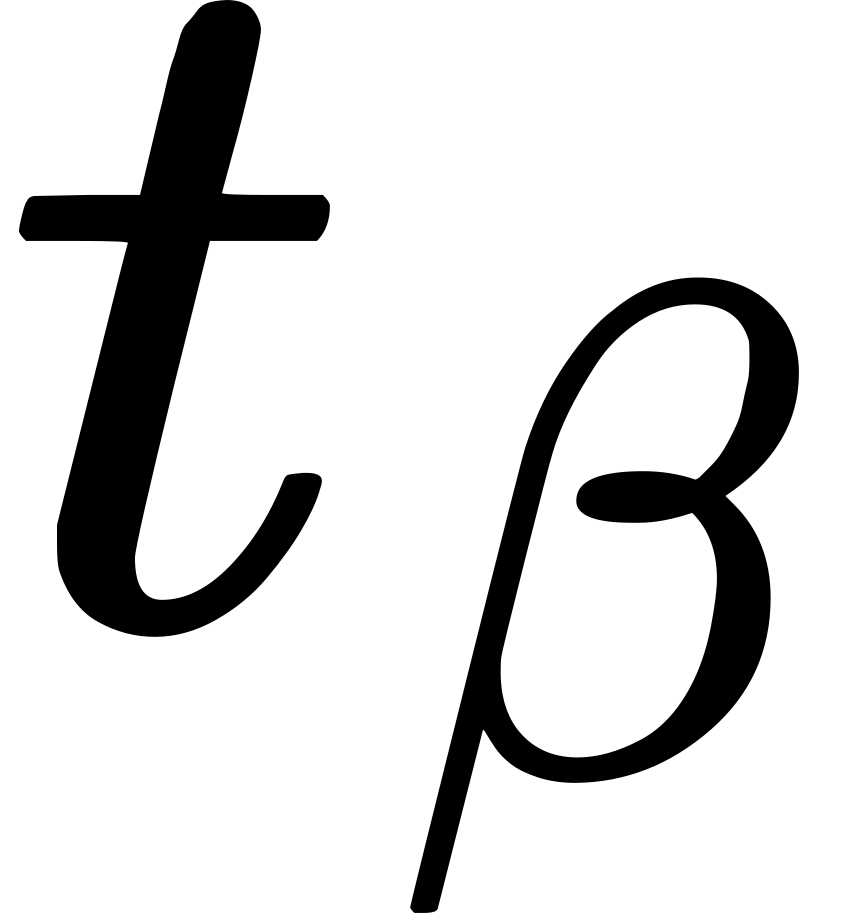 .
A pair of sets of four axes for a and allied as described in this
subarticle are called 'mutual axes' for the two systems.
49.7 The formulae for transformation from the
a-coordinates to the -coordinates, referred to mutual axes, are
obviously of the form
 where
 are constants dependent on the two systems and and
on the two arbitrarily chosen units of time-lapse in and
, but evidently not dependent on the arbitrarily chosen set of
rectangular rects and in the level
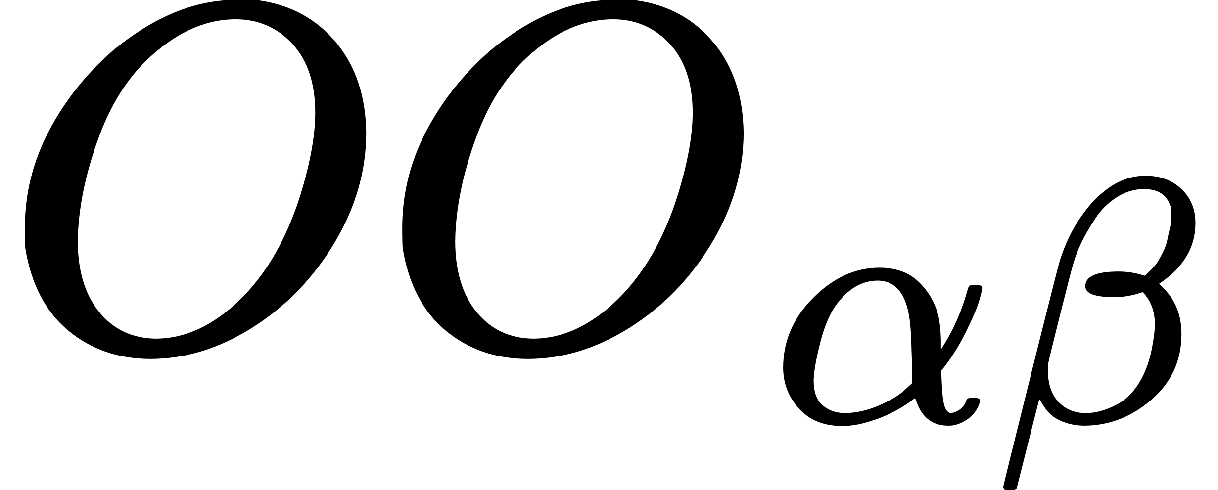 .
The corresponding (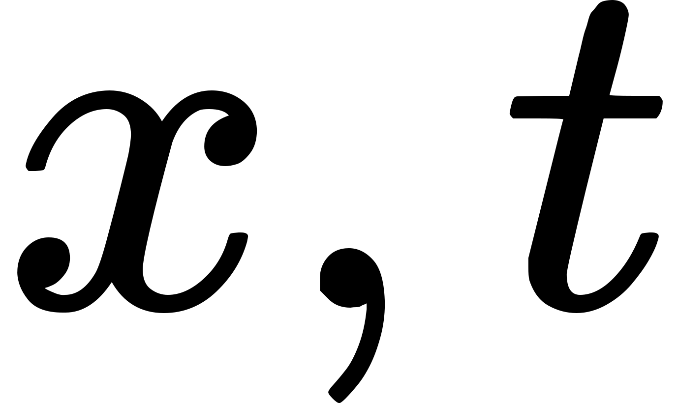 )-equations, interchanging and
, are

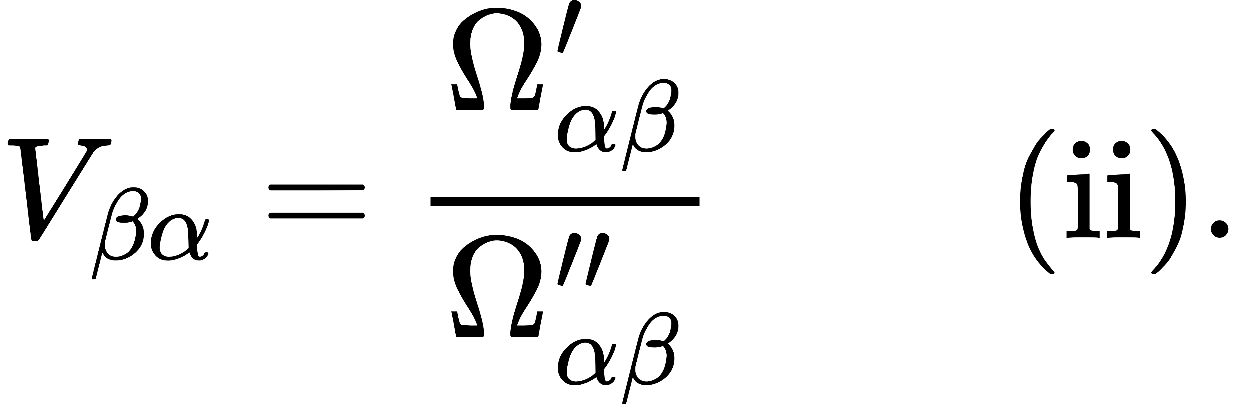
The two pairs of ()-equations, (i) and (ii), must be equivalent.
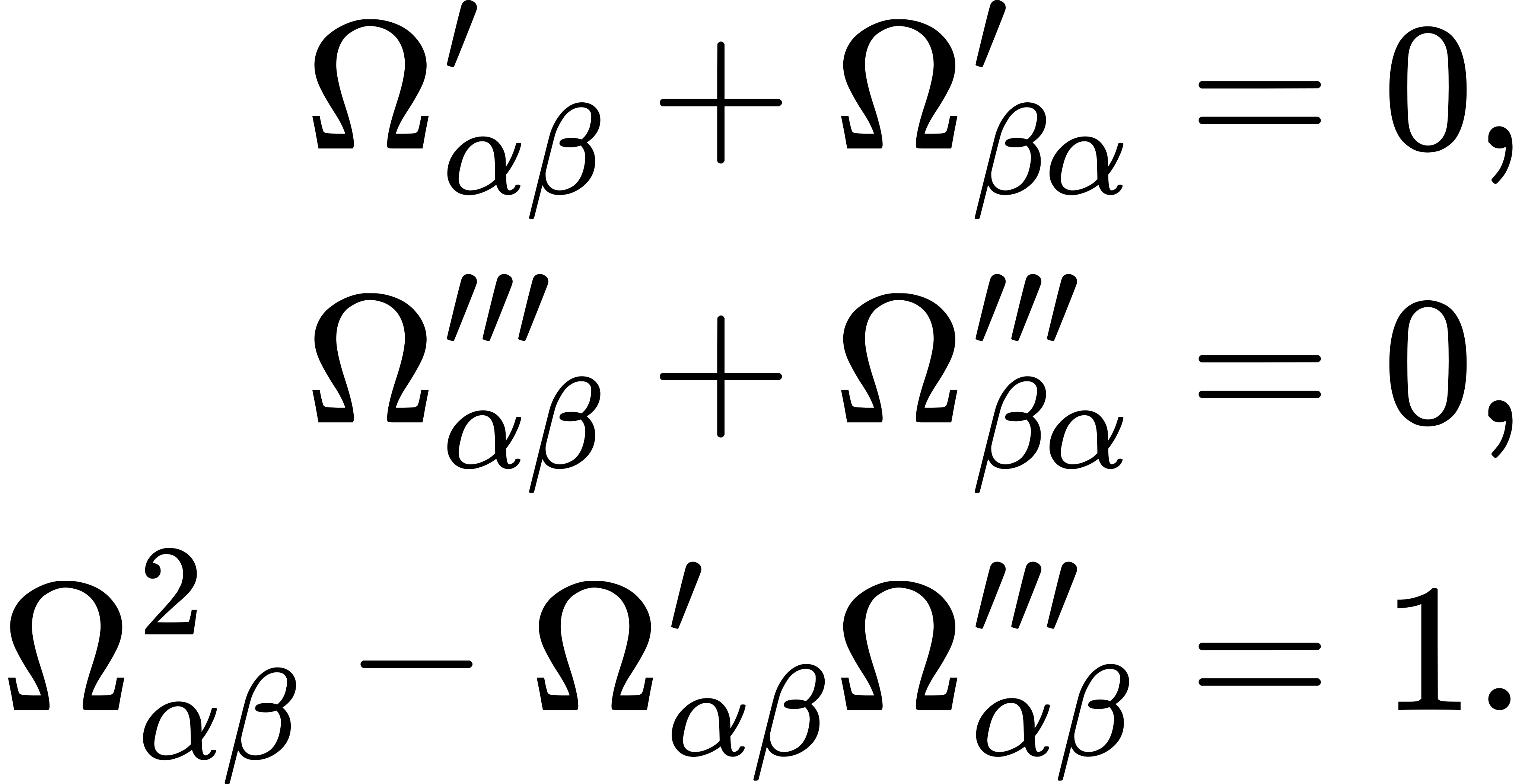
The conditions are

Only four out of these five conditions are independent.
50. The Principle of Kinematic Symmetry.
50.1 Consider any other time-system 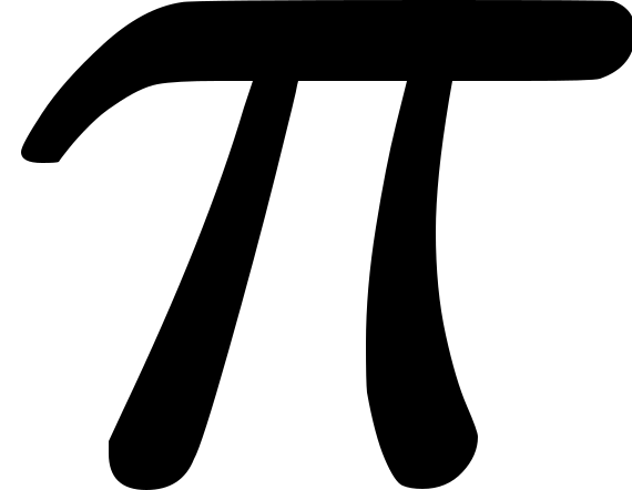 .
The -point (
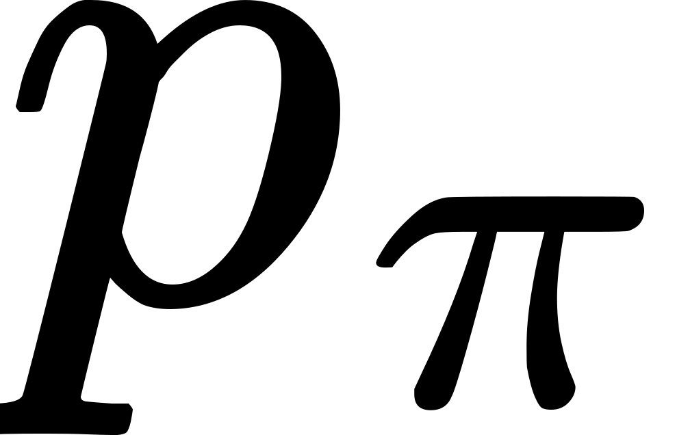 ) occupied by
()
and the -point occupied by the same event-particle lie on a
matrix
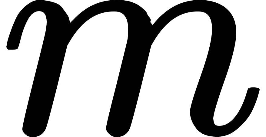 which includes an -line
(
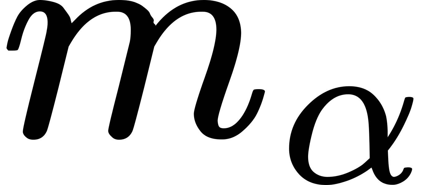 ) of which every -point is intersected by
. Thus correlates the -point
() with the -time
and the neighbouring -point on
namely
(
 ),
with the neighbouring -time
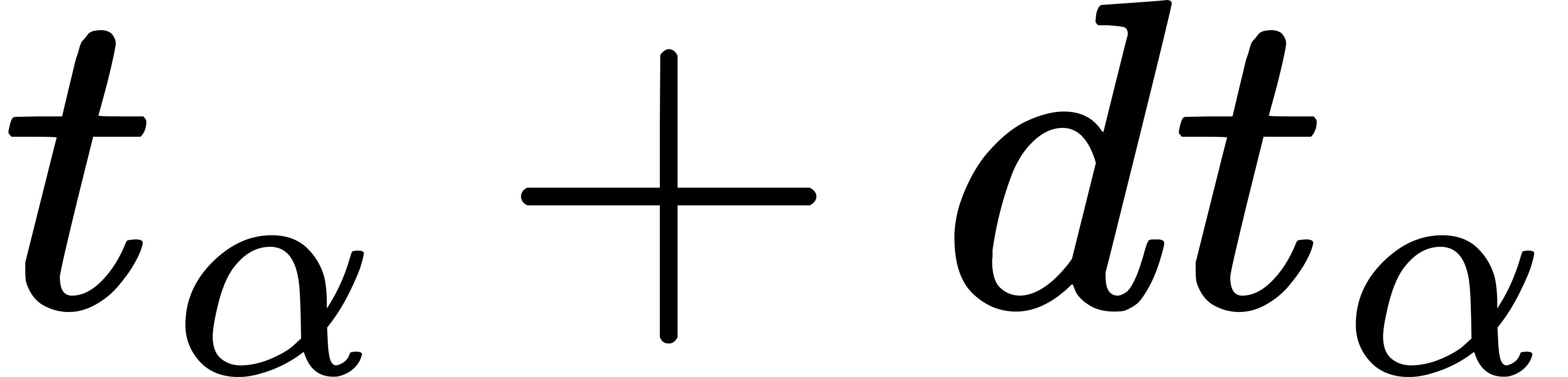 . In this way makes every set of
-coordinates of a variable -point to be a function
of ; namely it correlates an -point
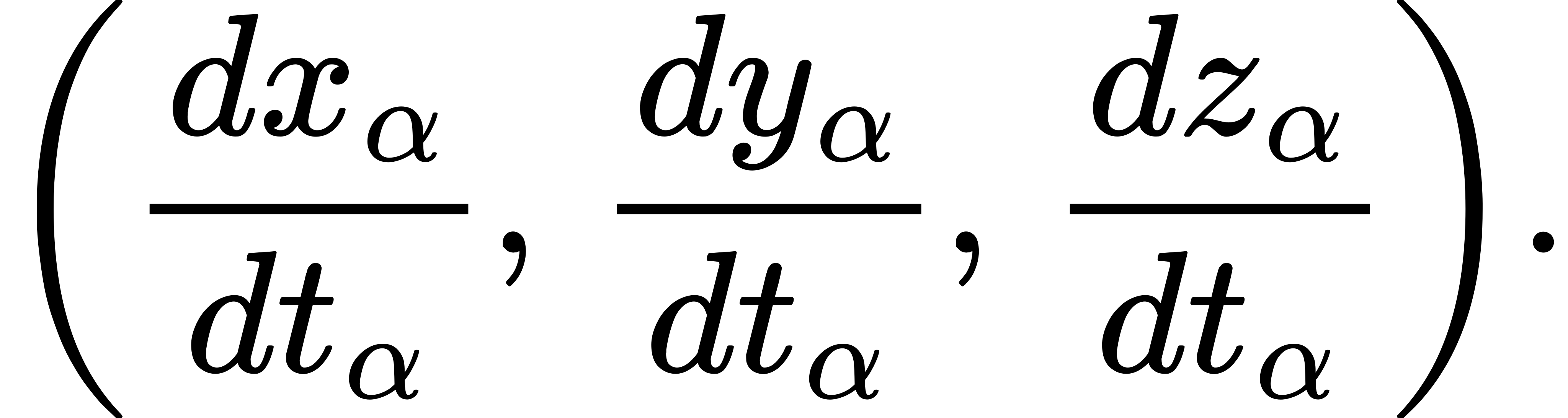
() with the velocity
(
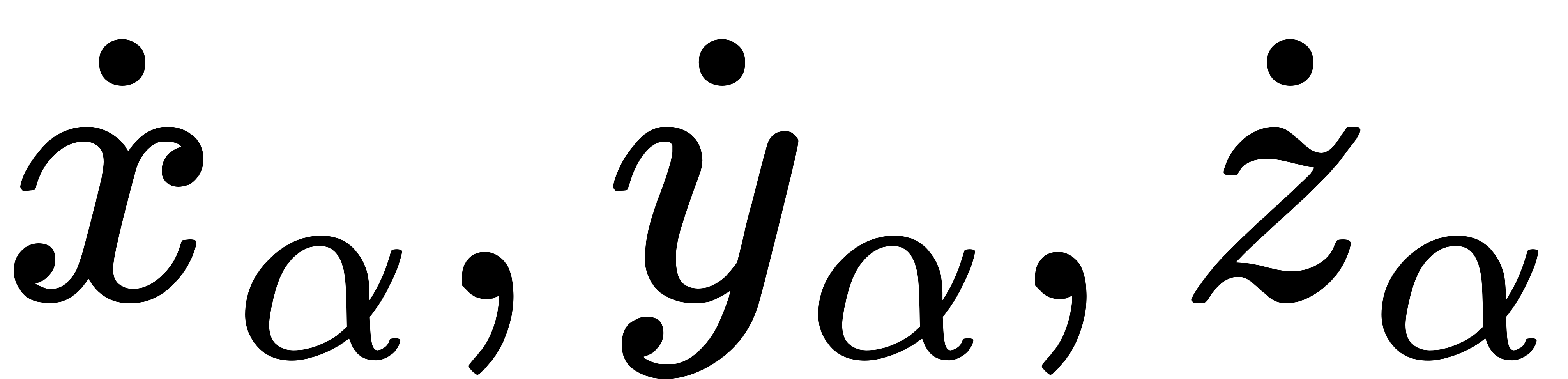 ), which can
also be written
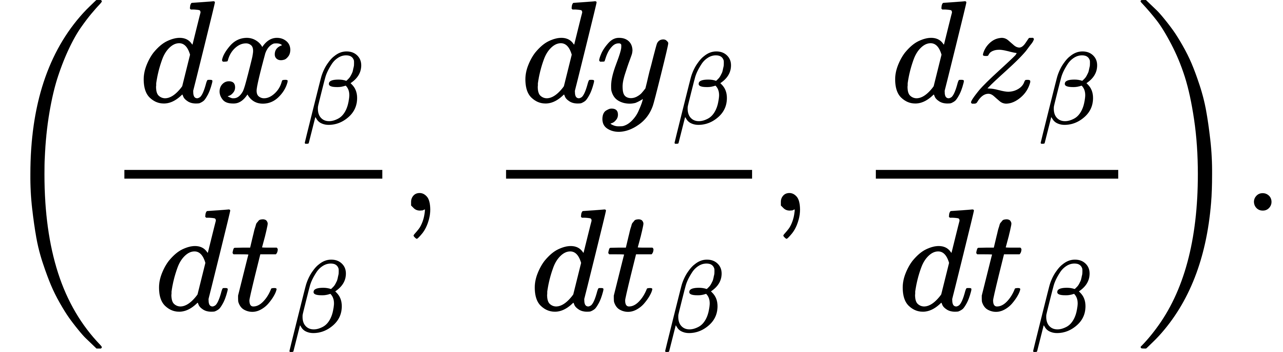
Analogously the same time-system correlates a -point
( ) with the velocity
(
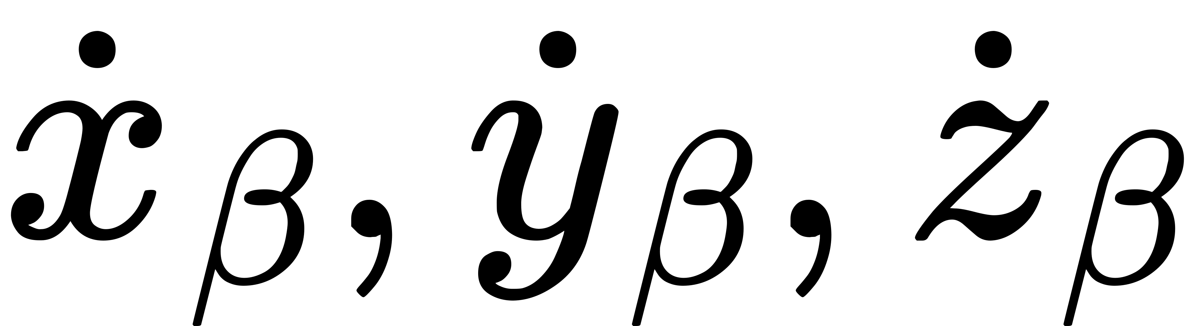 ) which can be
written
Now the time-system indicates a definite transference from an
event-particle ( ) to another
event-particle (
 )
occupying the same -point (
 ),
where any mutually normal -coordinates are employed. The former
event-particle is that indicated by
()
and by (), and the
latter event-particle by
(
 )
and by
(
 ).
Hence from equations (i) of 49.7

Now is any time-system. First identify it with .
Then  .
Hence
 , and
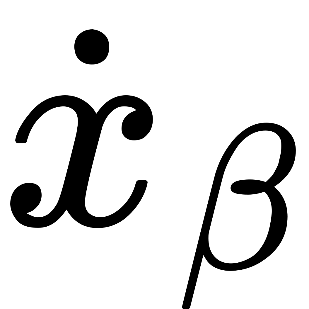 is the velocity of the time-system in the space of
[or, more briefly, the 'velocity of in ']. Let this
velocity be
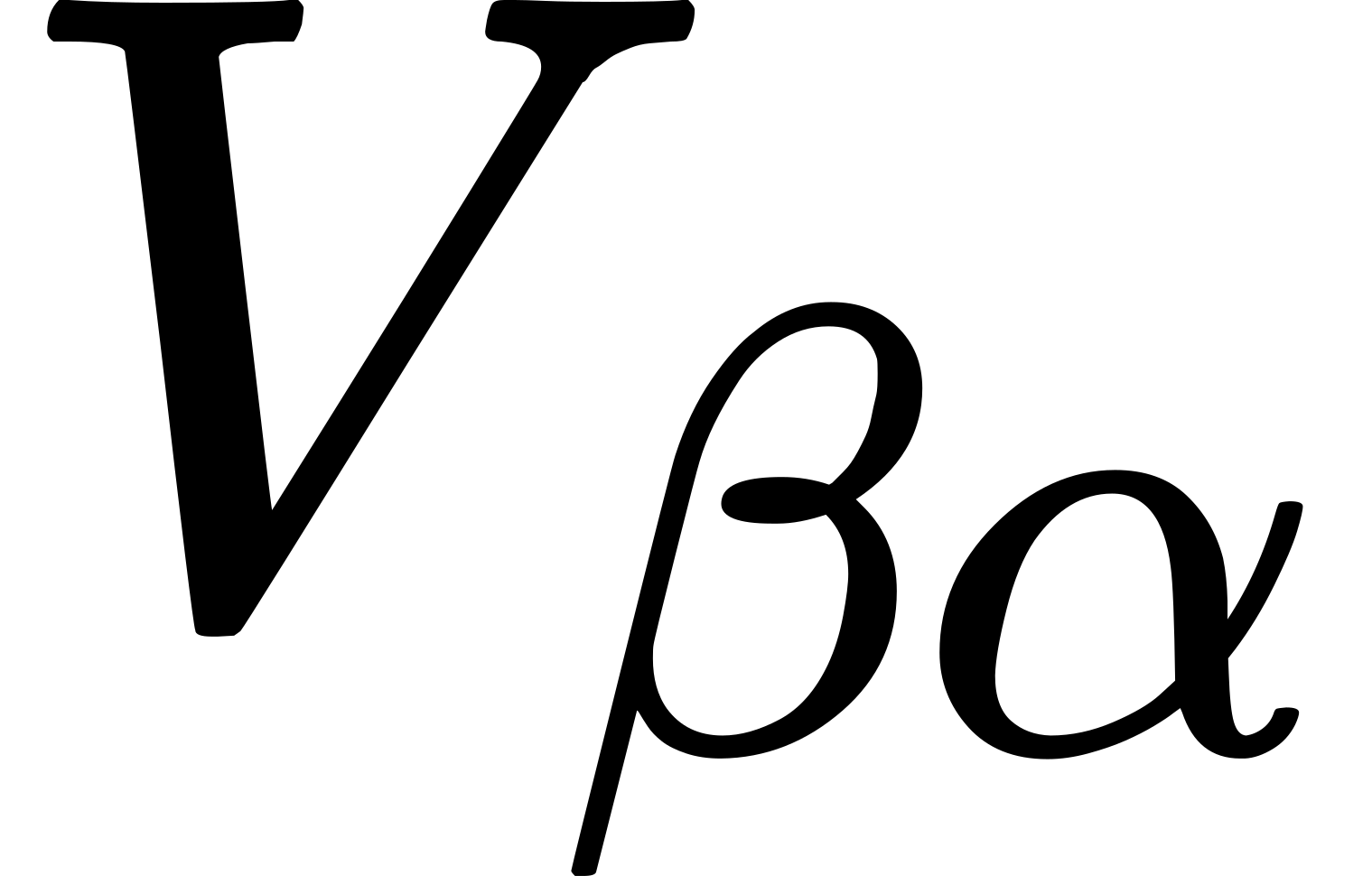 ; it is evidently along the
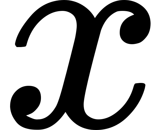 -axis in
the space of , and
 Again identify the system with . Then
 ;
and hence
 , and
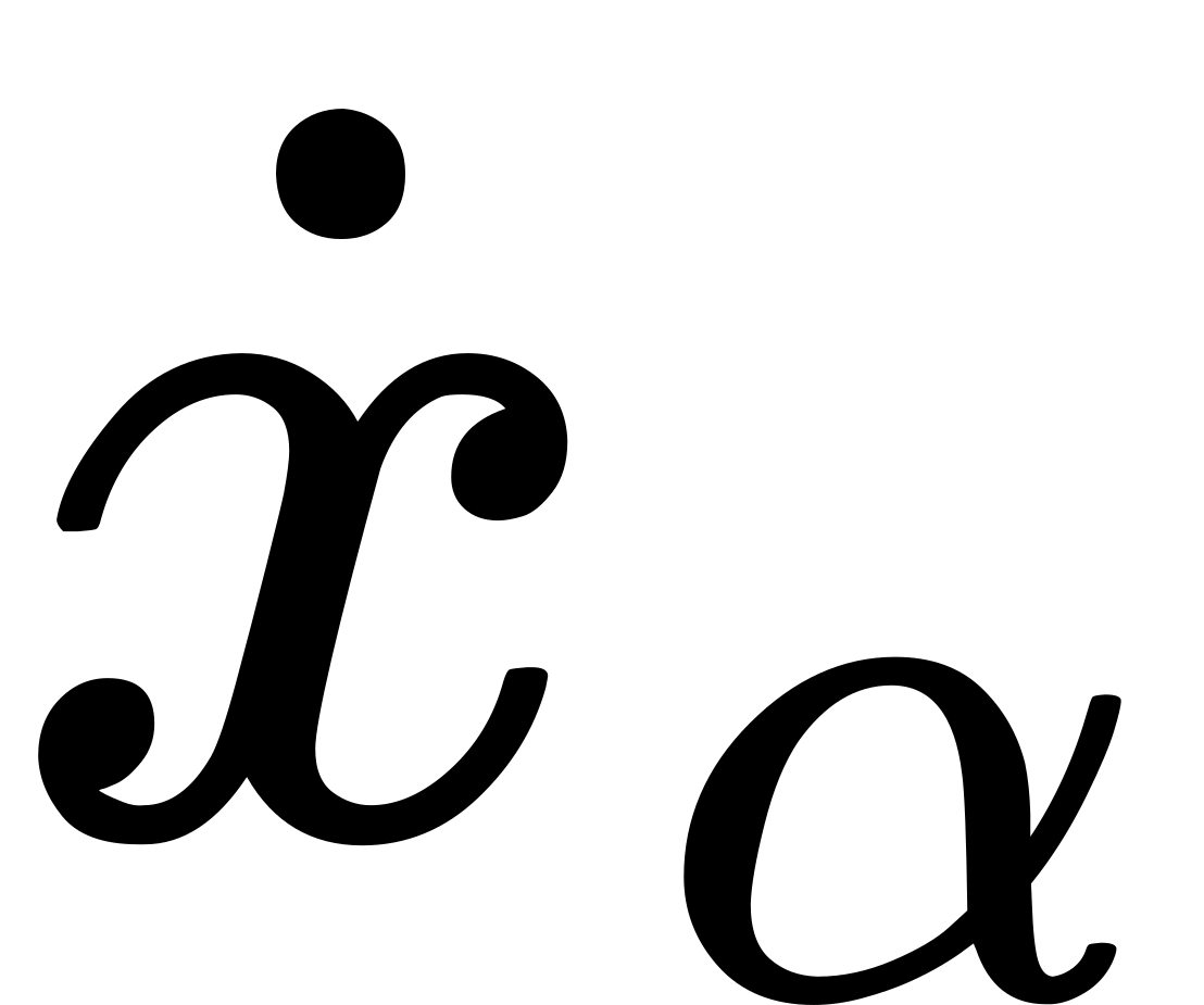 is the velocity of in . Let this
velocity be
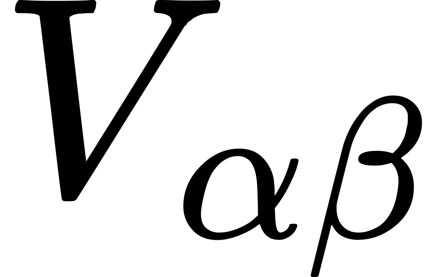 ; it is along the -axis in the space
of , and
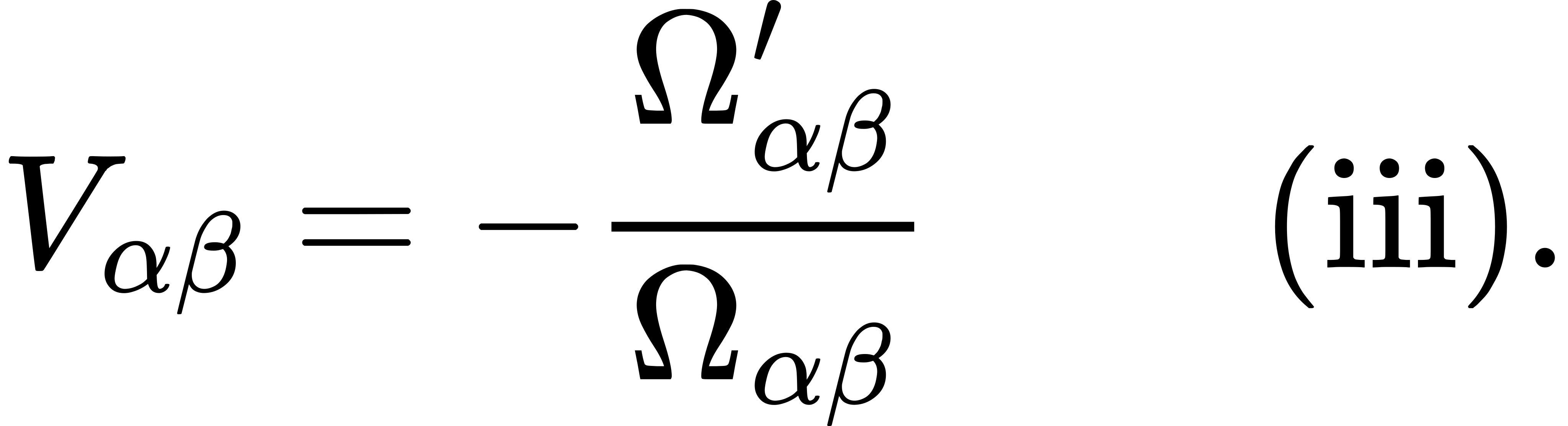
50.2 We will now introduce what we will term the 'Principle of
Kinematic Symmetry.'
Before enunciating this principle it is necessary to determine a
standard method of choosing the positive directions of the axes
and in the matrix
and of the axes
and . By reference to the figure of
subarticle 45.2 it will be seen that, of the four
angular regions into which the rects and
divide the matrix , two vertically opposite regions
include no point-tracks passing through and the remaining two such
regions include point-tracks as well as rects through . The standard
choice of positive directions for and is
such that the two regions bounded one by both positive directions of
these axes, and the other by both negative directions, should include
only rects passing through .
The positive directions for and are
settled by the rule that a positive measure of lapse of time should
indicate subsequence in the time-order to the moment .
This rule is definite because of the ultimate distinction between
antecedence and subsequence in time, which has not otherwise been made
use of. This standard choice of positive directions along mutual axes
for two time-systems will always be adopted.
50.3 The principle of kinematic symmetry has
two parts, enunciating consequences which flow from the fact that the
time-units in two time-systems and are congruent.
The first part may be taken as the definition, or necessary and
sufficient test, of such congruence.
The first part of the principle can be enunciated as the statement that
the measures of relative velocities [i.e. the velocity of in
and of in ] are equal and opposite;
namely

The second part is the principle of the symmetry of two time-systems in
respect to transverse velocities; namely, if a velocity 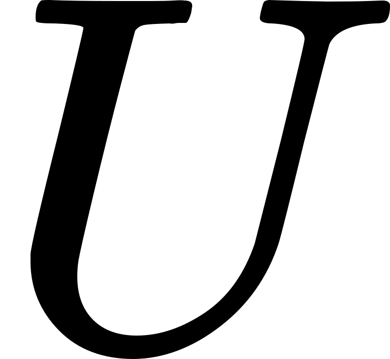 in
, normally transverse to the direction of in
, is represented by the velocity (
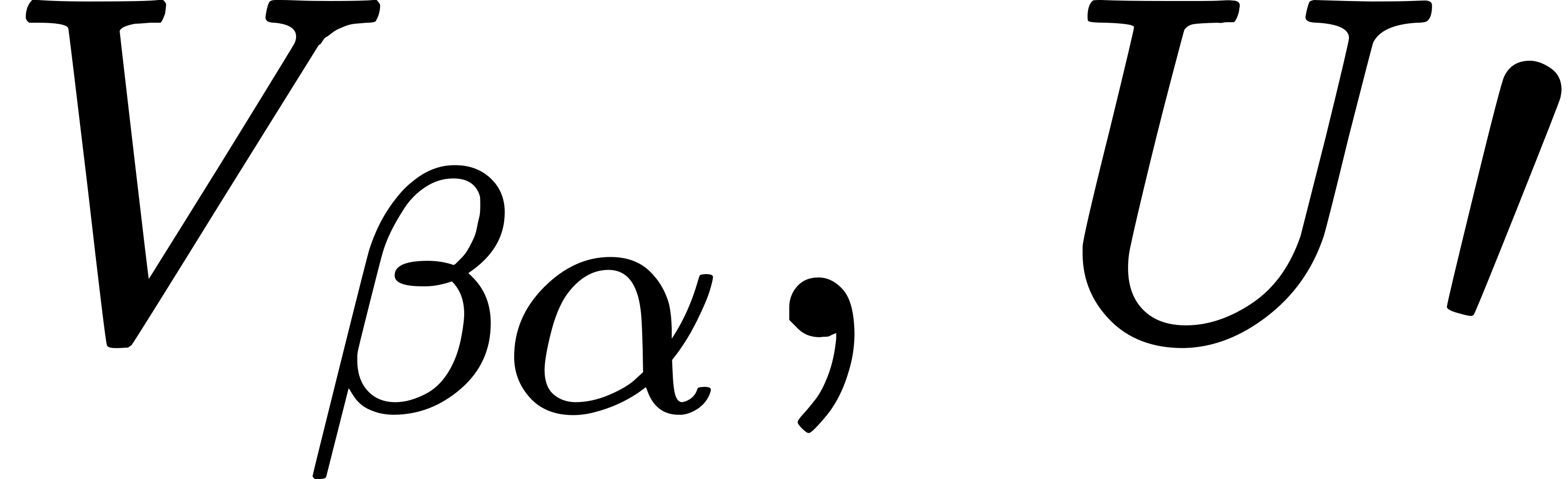 )
in , where is along the direction of
in and ′ is normally transverse to it, then
the same magnitude of velocity in , normally transverse
to the direction of in , is represented by the
velocity (
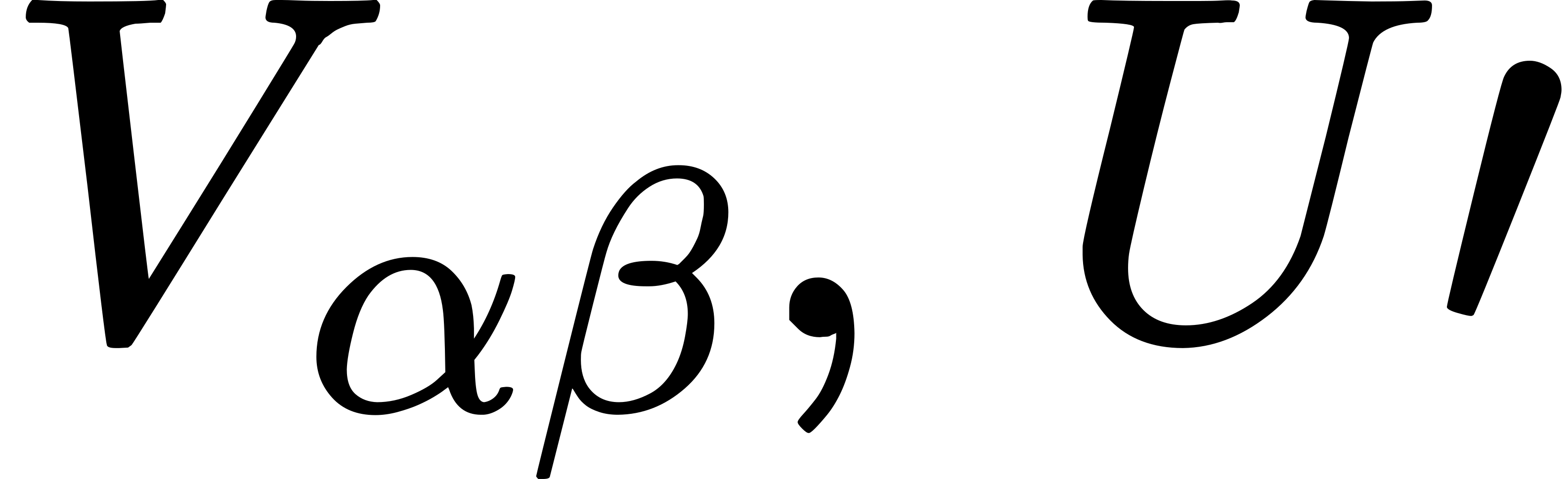 ) in , where
is along the direction of in ,
and ′ is normally transverse to it.
From the first part of the principle, by (ii) and (iii) of
50.1, we deduce
 In order to apply the second part of the principle we first identify
with
 ),
then from (i) and (ii) of 50.1
 Again we identify
( with
 ), and
by interchanging and in the above formulae we find
 Hence by the second part of the principle

51. Transitivity of Congruence.
51.1 It follows, from (iii) of
49.7, and from (ii) and (iii) of
50.1, and from (i), (ii), (iii) of
50.3, that equations (i) of
50.1 can be written


We can now express 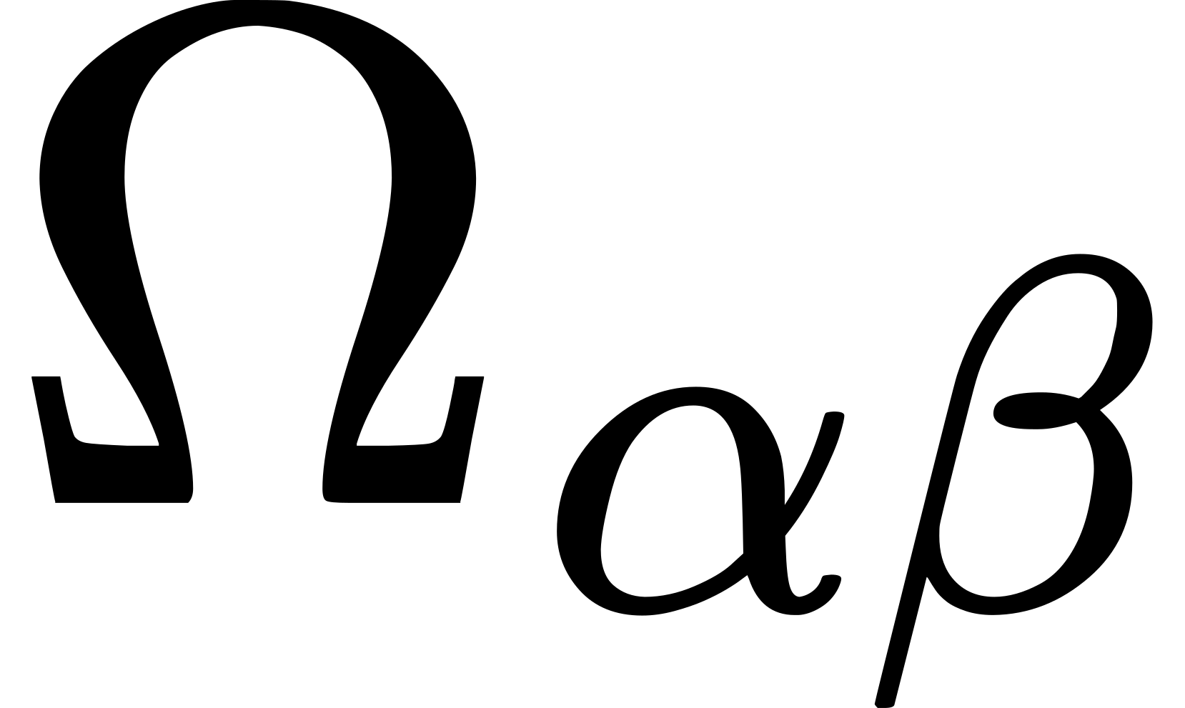 and
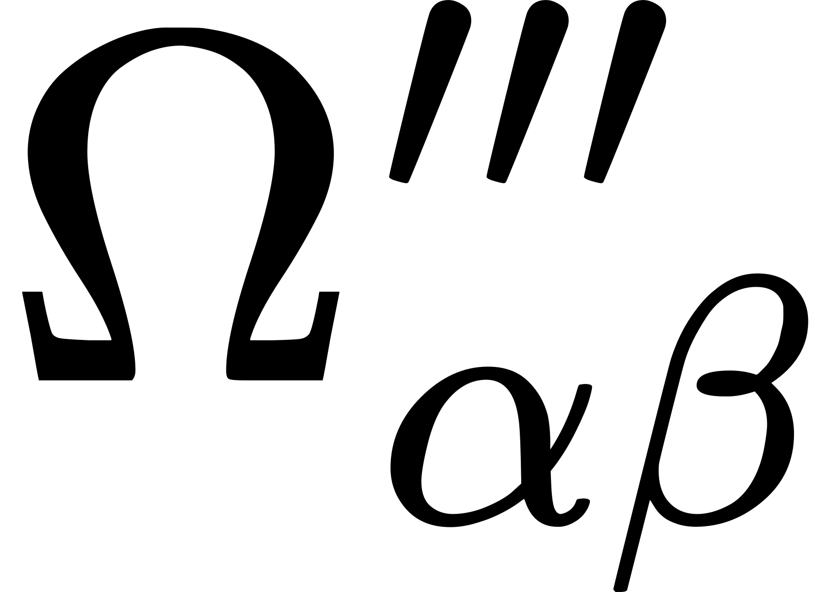 in terms of
and an absolute constant by considering deductions
from the transitivity of congruence.
51.2 Let 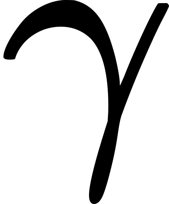 be a time-system such
that the level
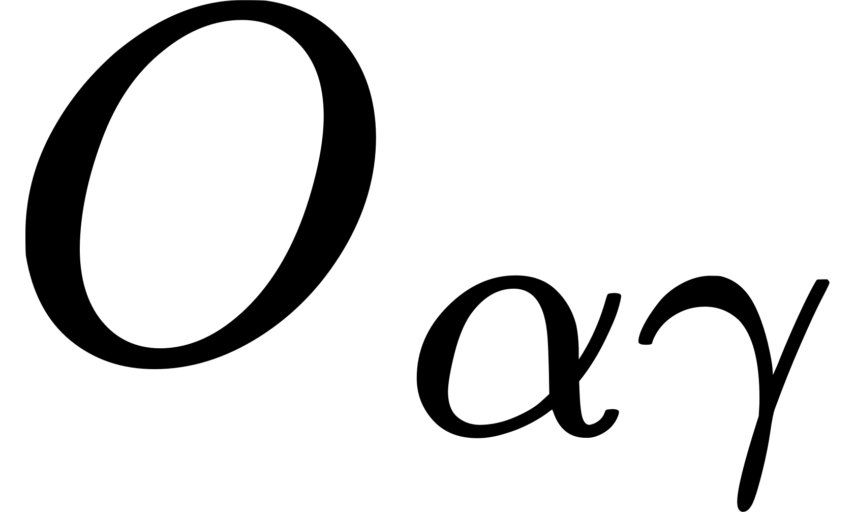 contains and
, and let these rects be the axes
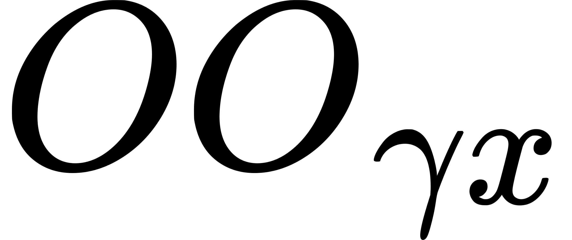 and
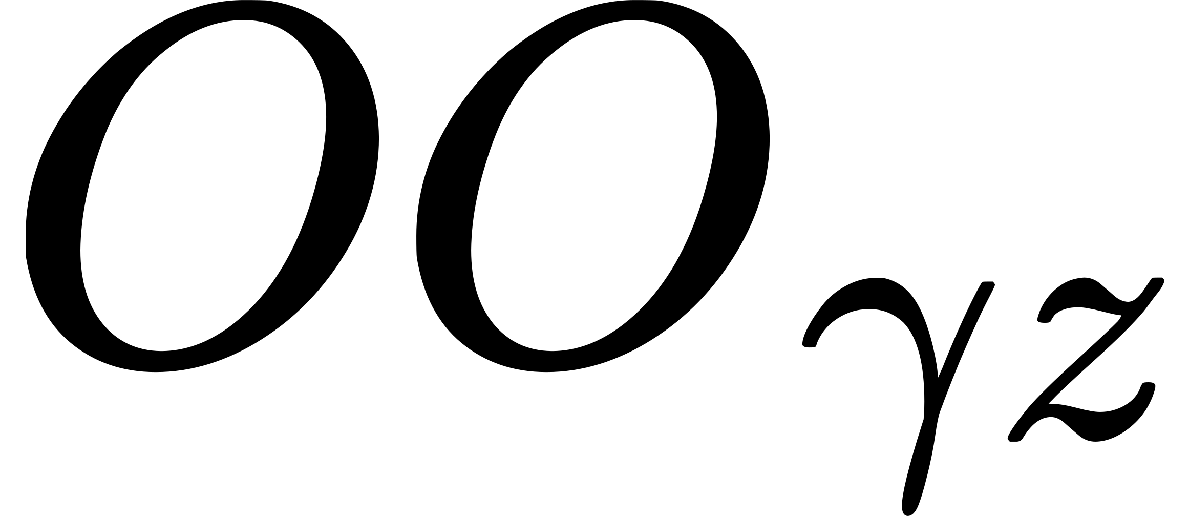 . Then the matrix
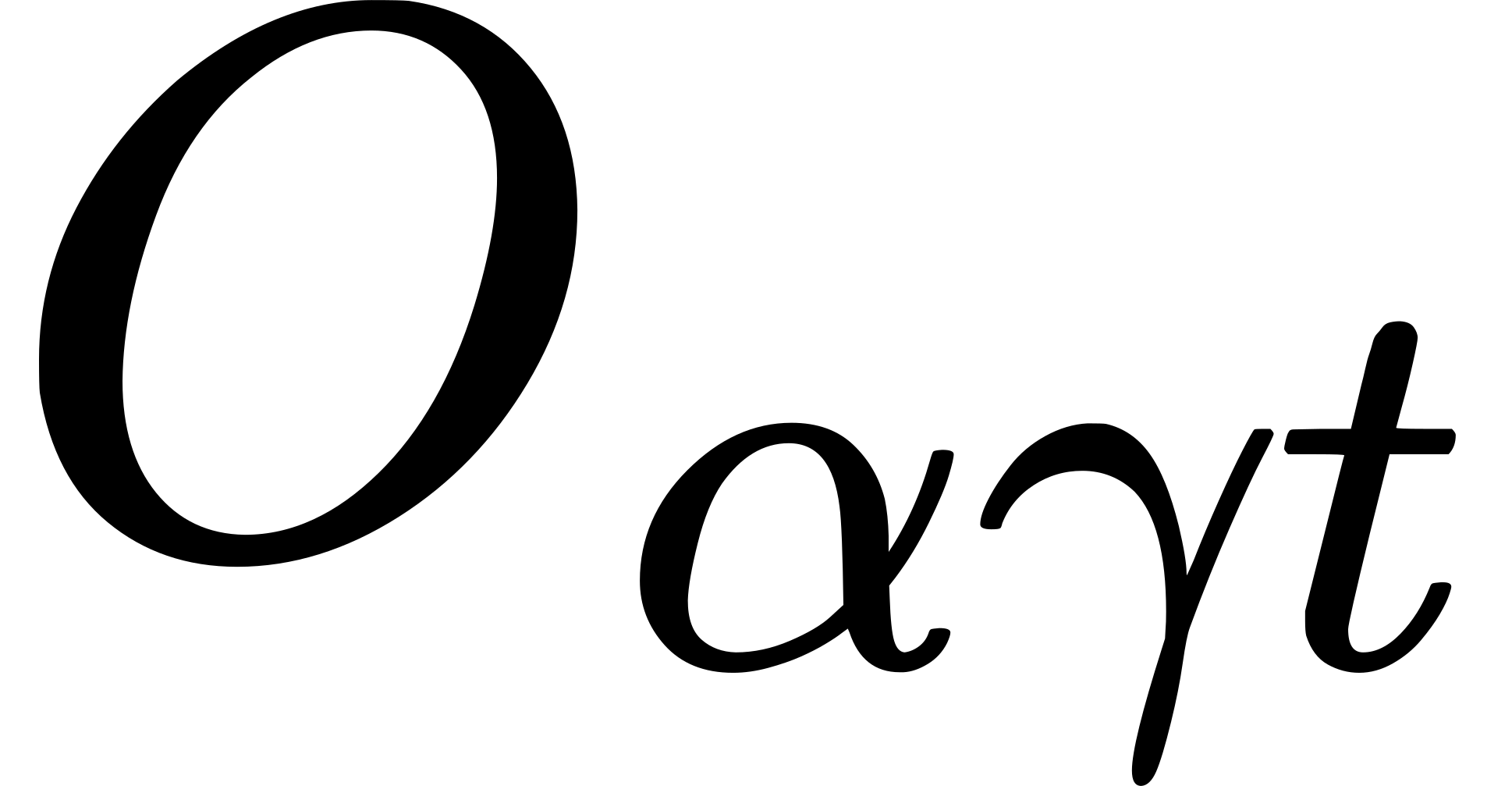 contains
,
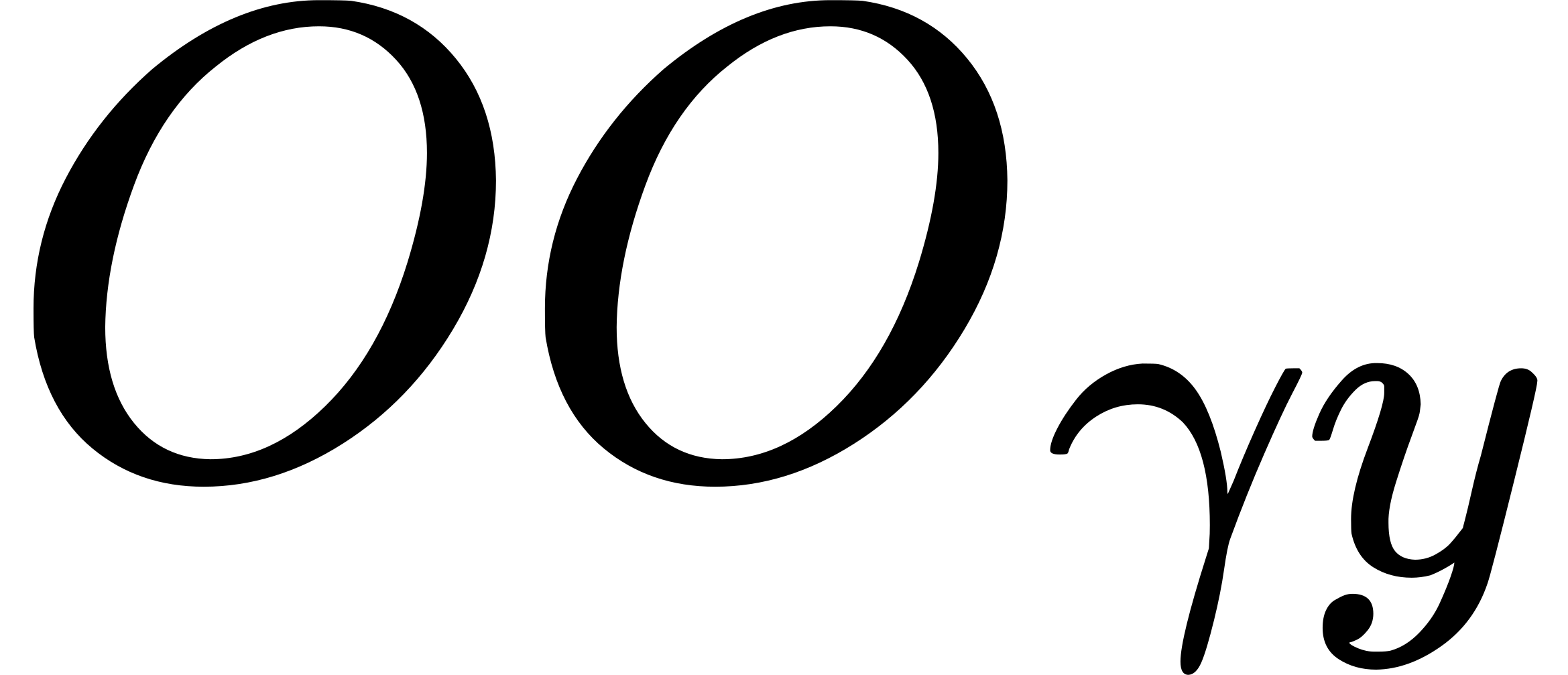 , and
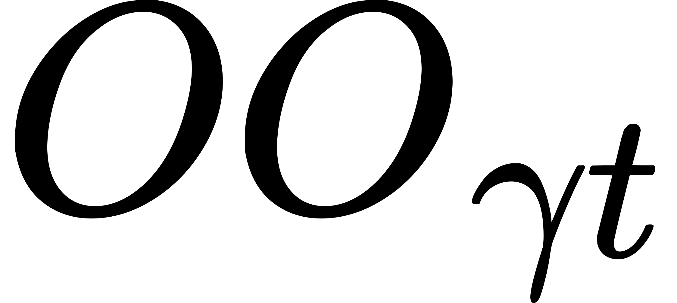 . Thus we have obtained a set of mutual axes for
and ; namely,
() and (
 ),
where and now play
the part that and sustain for
and . Thus the velocities of the time-system
in and are, by (i) of 51.1,
connected by

We have here assumed the congruence of the time-units in and
.
Now identify and . Then

Hence from (i) of 51.1



Again identify with . Then

Hence from (i) of this subarticle



From (ii) and (iii) and (i) of 50.3
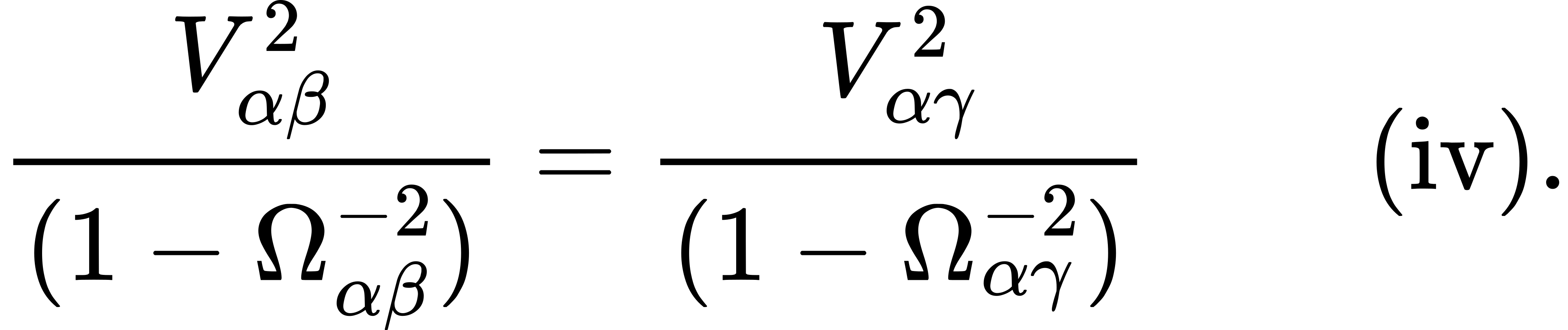
51.3 Evidently if 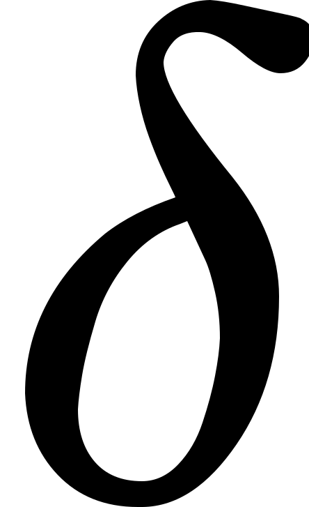 be any other member
of the collinear set of time-systems (, ), then
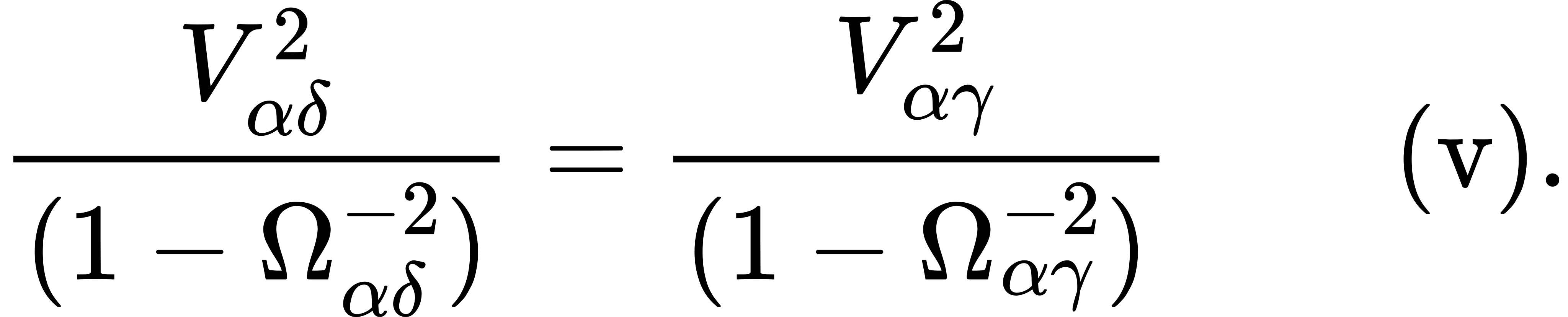
Hence if 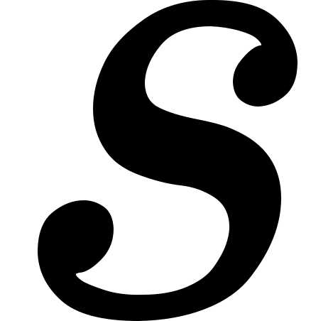 be a collinear set of time-systems, and
, , ,
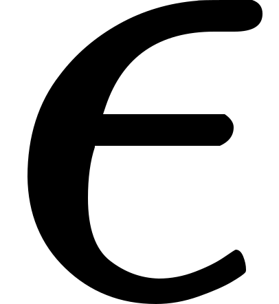 be any four of its members,
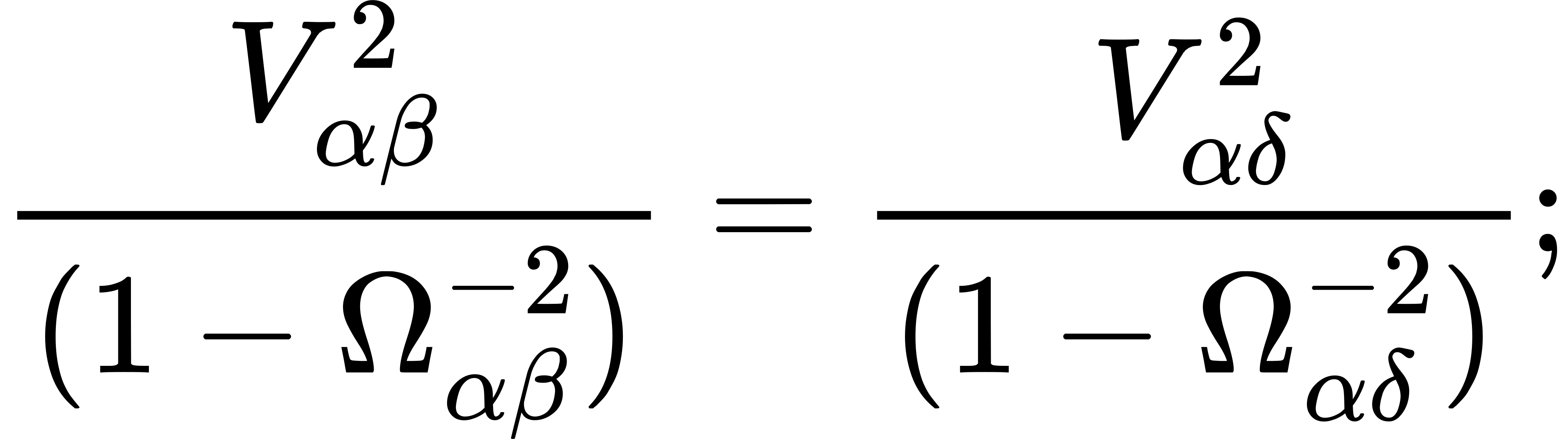 and hence, since
 , we
obtain
 where
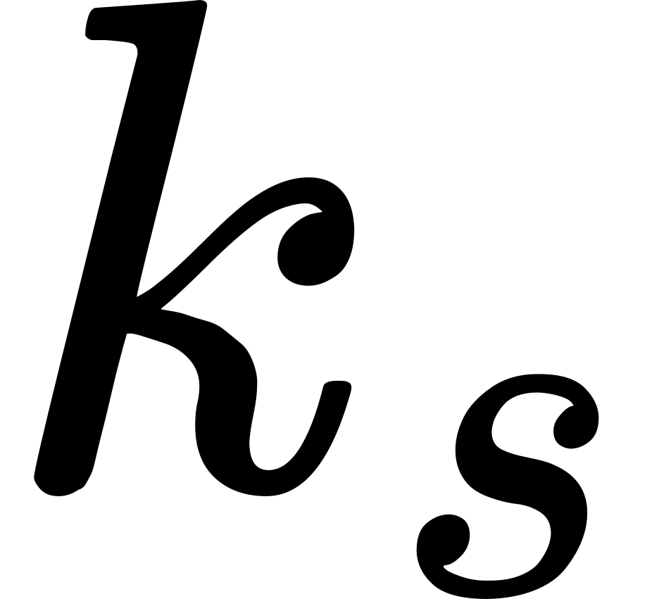 is a constant for the collinear set.
Furthermore, if be a time-system not belonging to but
related to and as explained in 51.2,
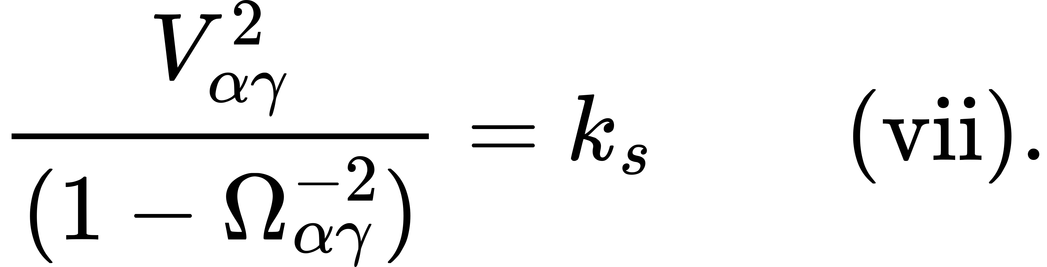
51.4 Now let , , 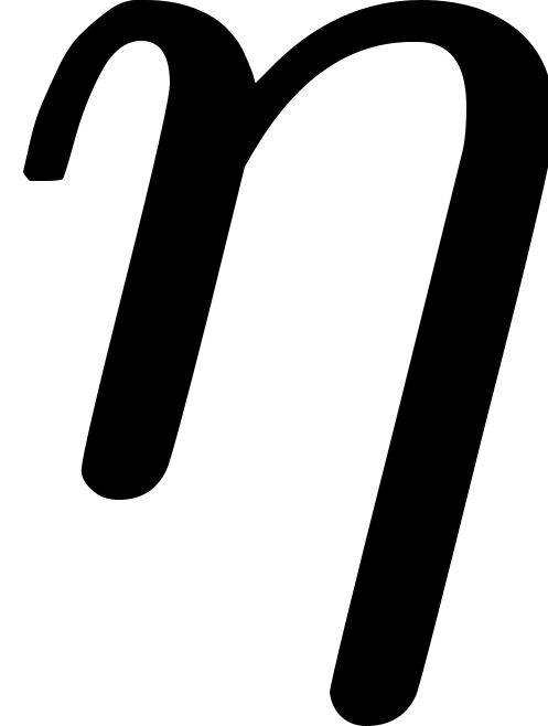 be any three
non-collinear time-systems, and construct a diagram to represent
elements in the time-less space of according to the familiar
method of geometricians.
The points of the diagram symbolise -points, and the straight
lines of the diagram symbolise -lines. Let be any
-point and let 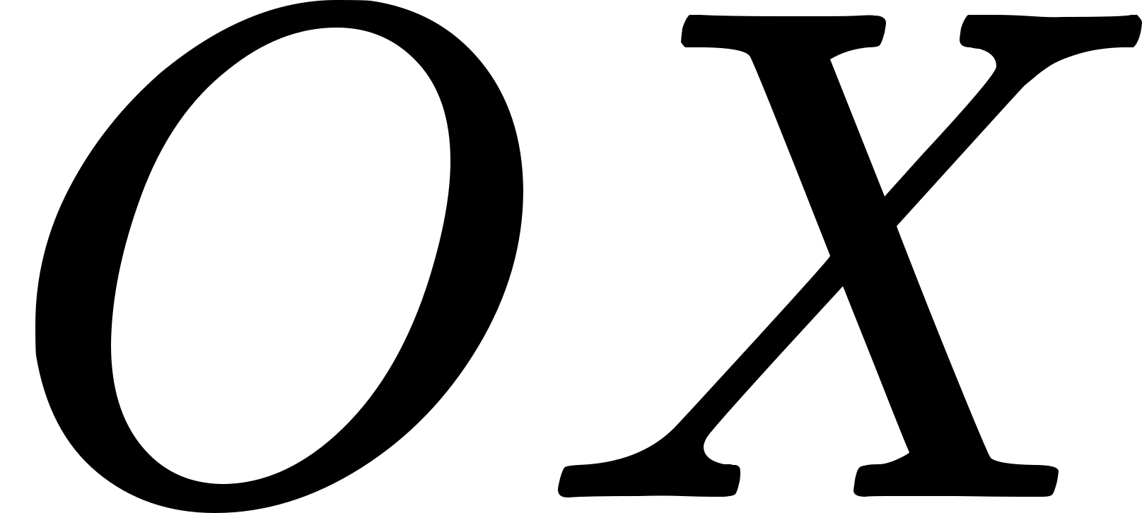 be the direction in -space
of the velocity . Then is the direction in
-space of the velocity (positive or negative) of any member of
the collinear set (
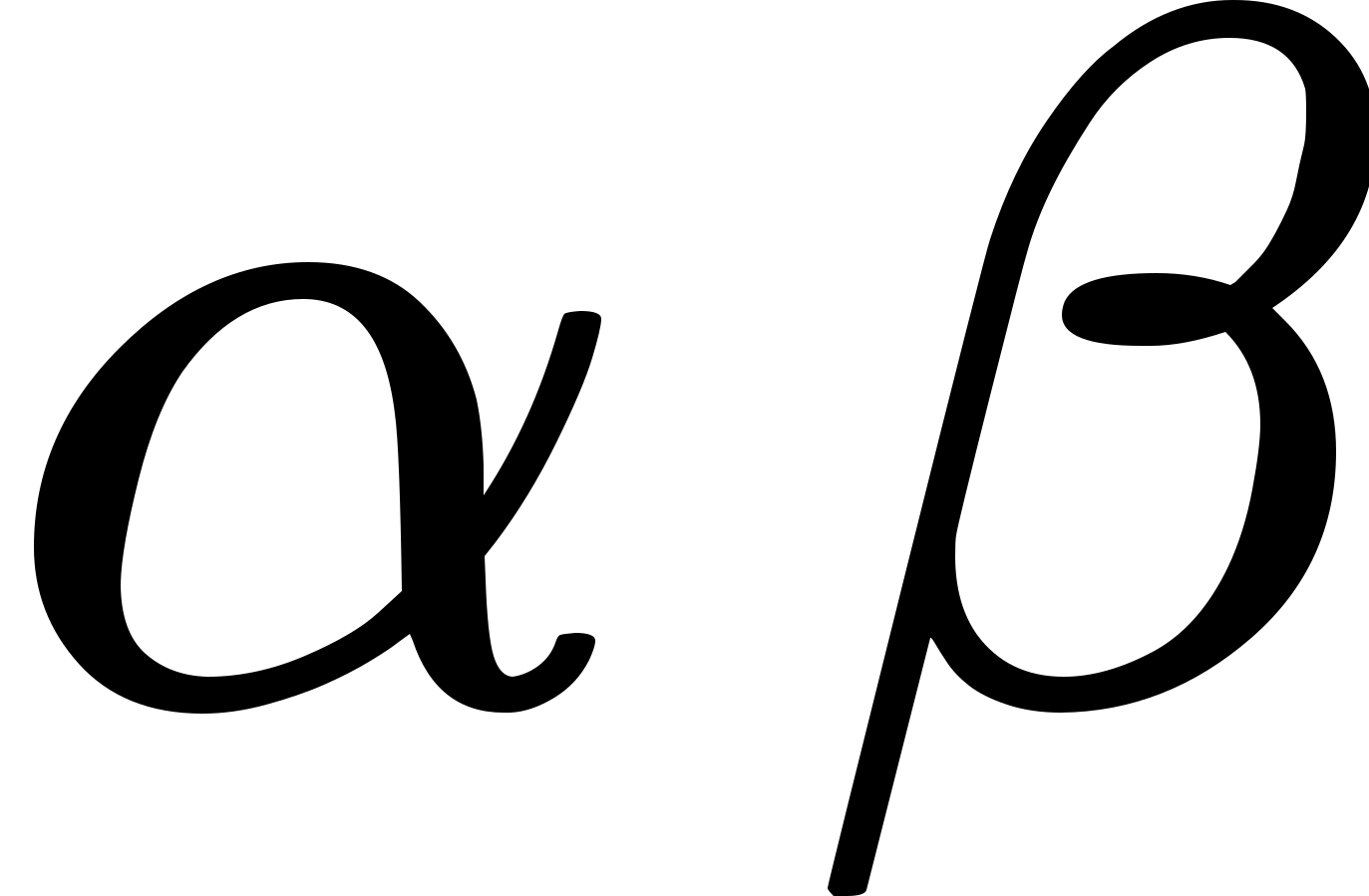 ).
Let 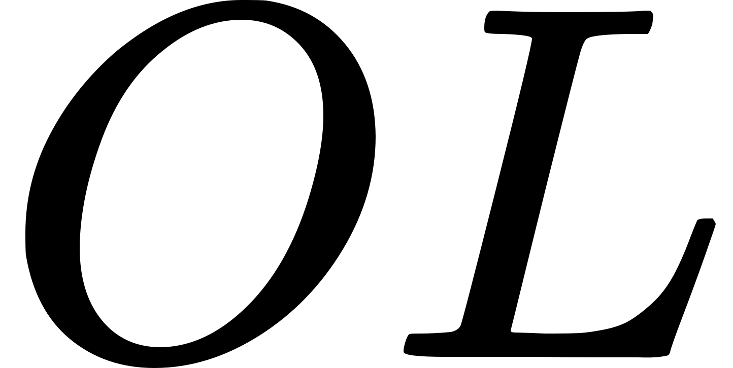 be the direction in -space of the velocity
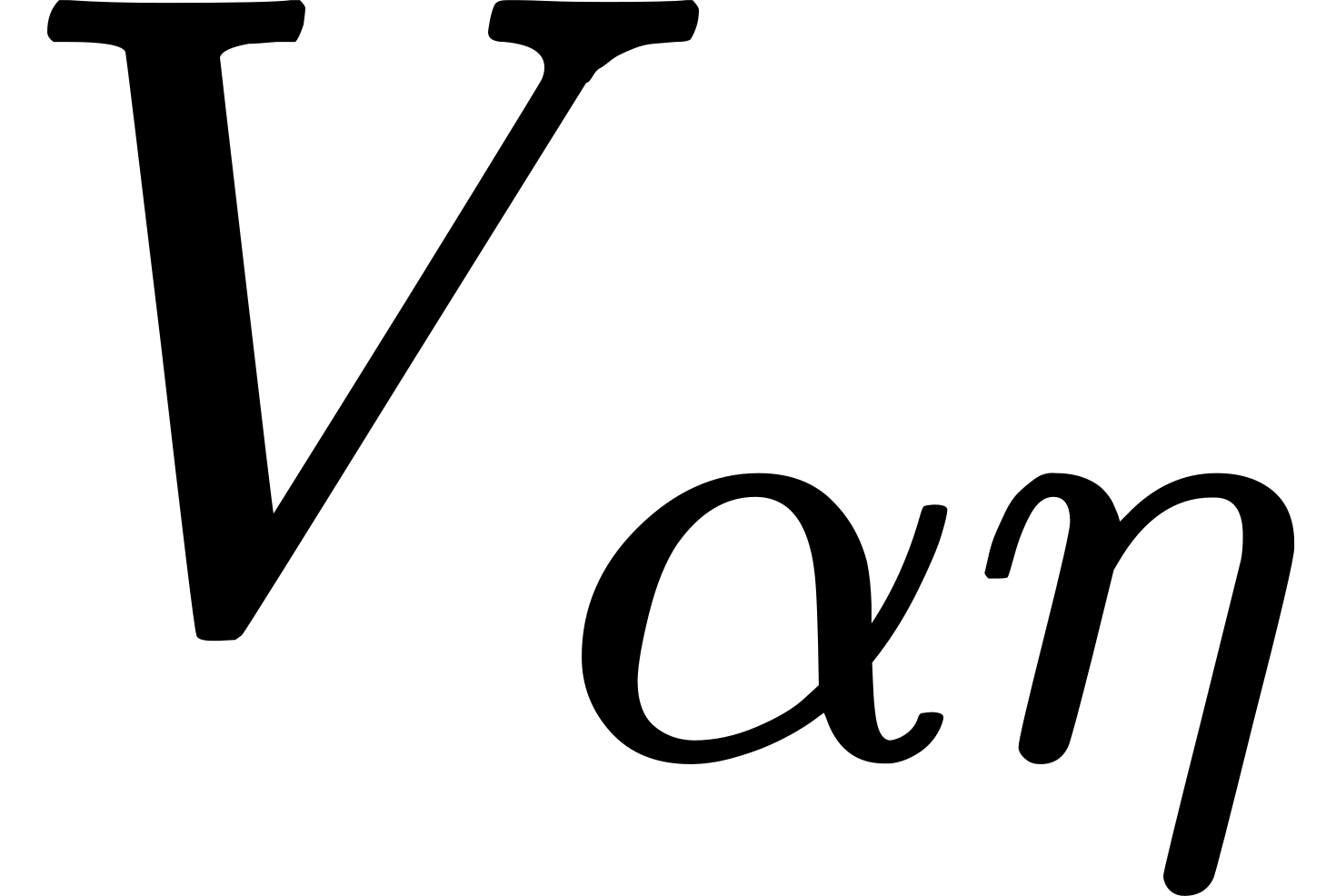 ; by hypothesis is distinct from . Let
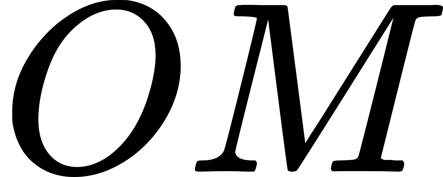 be the -line perpendicular to the -plane
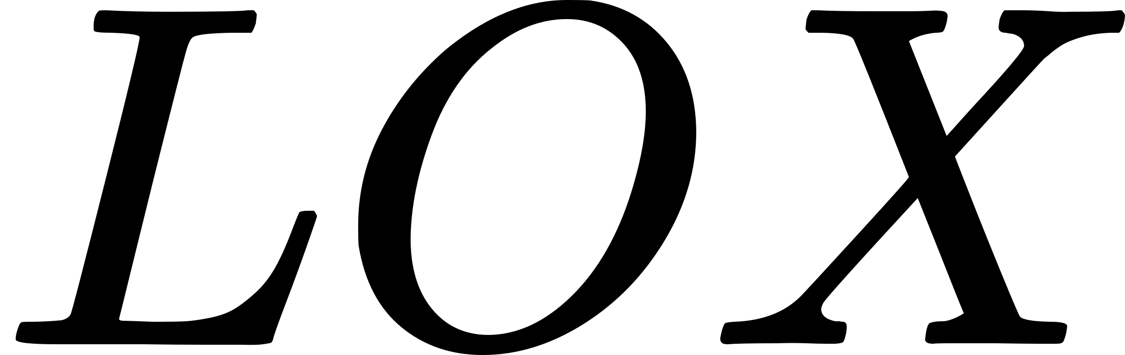 , and let be a time-system whose velocity in ,
namely
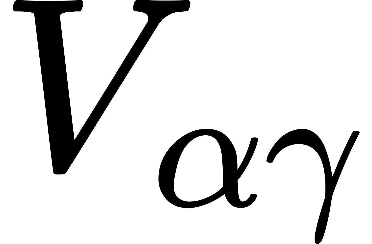 , is along . Let denote the
collinear set (), ′ the collinear set
(
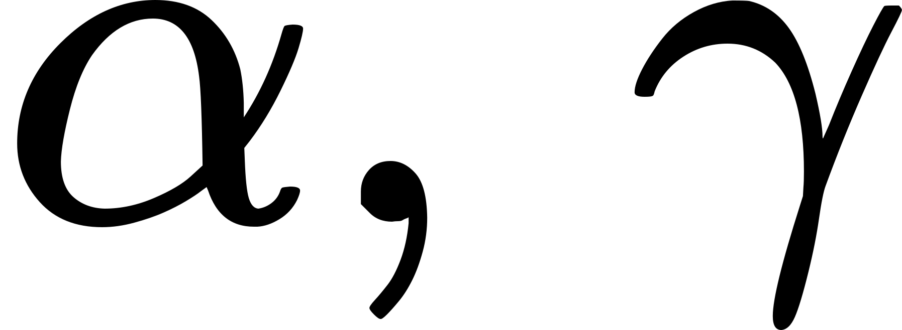 ), and ″ the collinear
set (
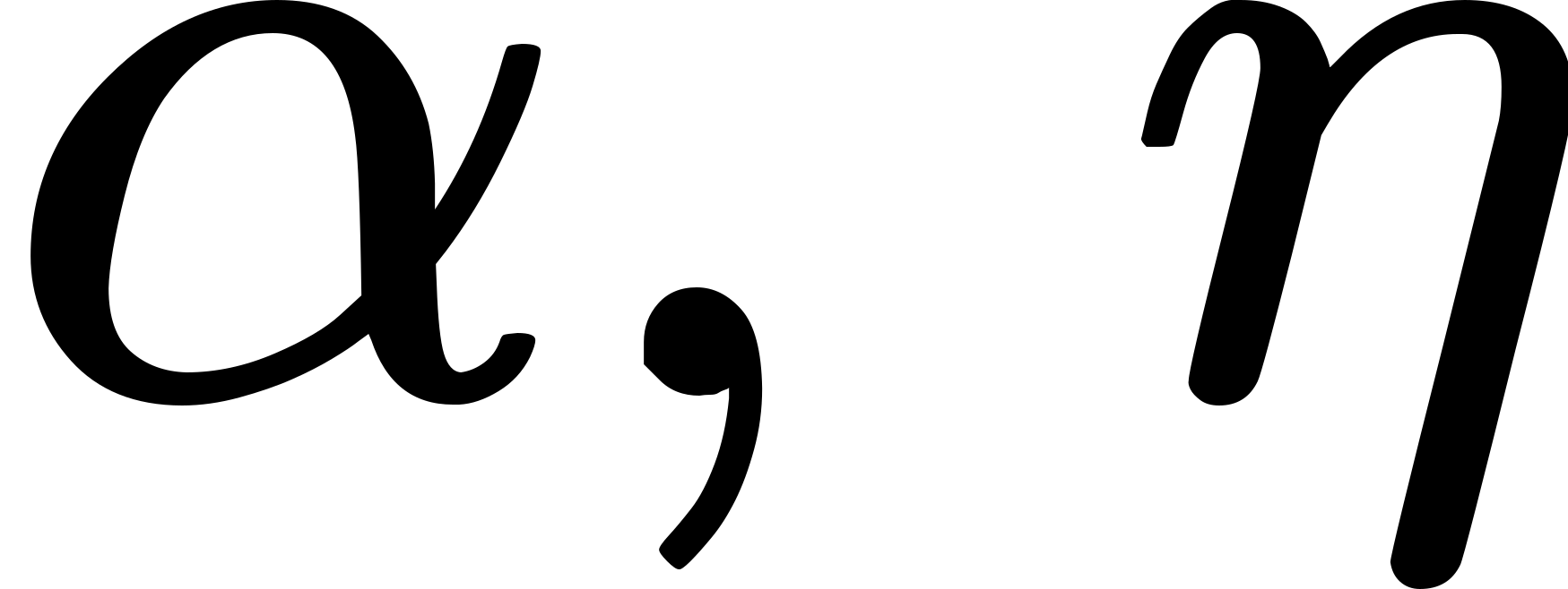 ). Hence from (vi) of 51.3

Hence from (vii) of 51.3


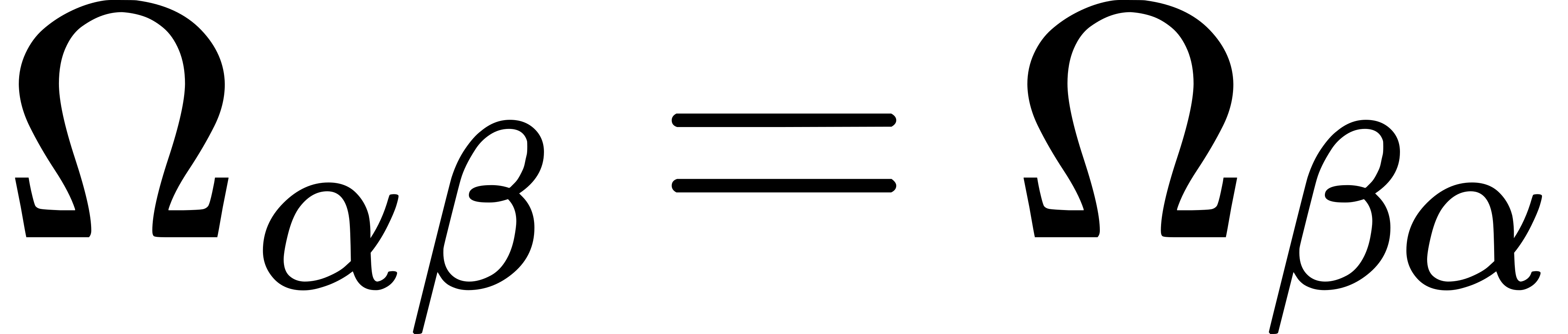
Hence, since 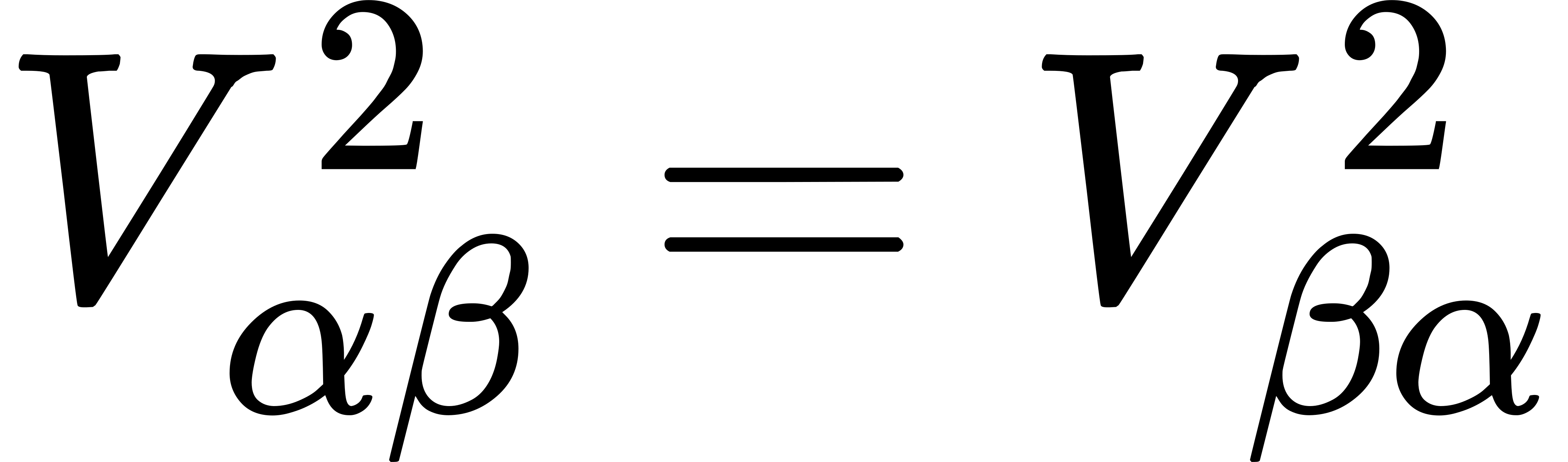 and
 , it is easy to prove
that is the same for any pair of time-systems; in other words,
that is an absolute constant.
52. The Three Types of Kinematics.
52.1 There are thus three types of kinematics possible, according
as is positive, negative, or infinite. The formally possible
type where is zero requires that either or
should be zero; by reference to (i) of
49.7 and to (i) of 51.1 this
supposition is seen to lead to results in such obvious contradiction to
experience as to preclude the necessity for further examination. Let us
name the types retained (according to the familiar habit) the
'hyperbolic,' the 'elliptic' and the 'parabolic' types of kinematics.
52.2 First consider the hyperbolic type and
put 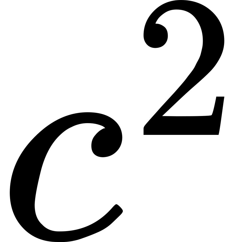 for . The equations of articles
49 and 51 then become


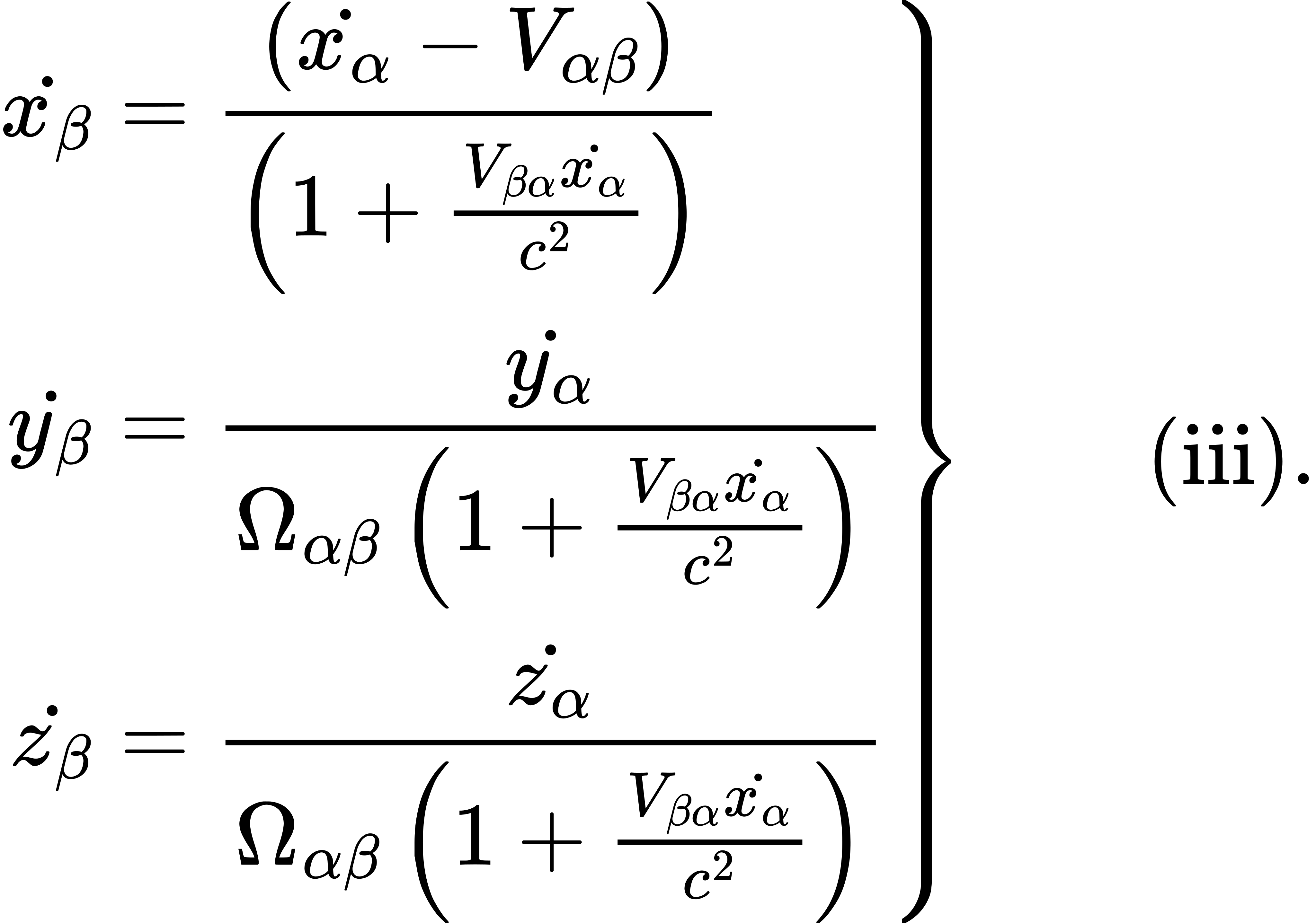
The equations of transformation, namely (ii), can be expressed
symmetrically as between and by means of the scheme
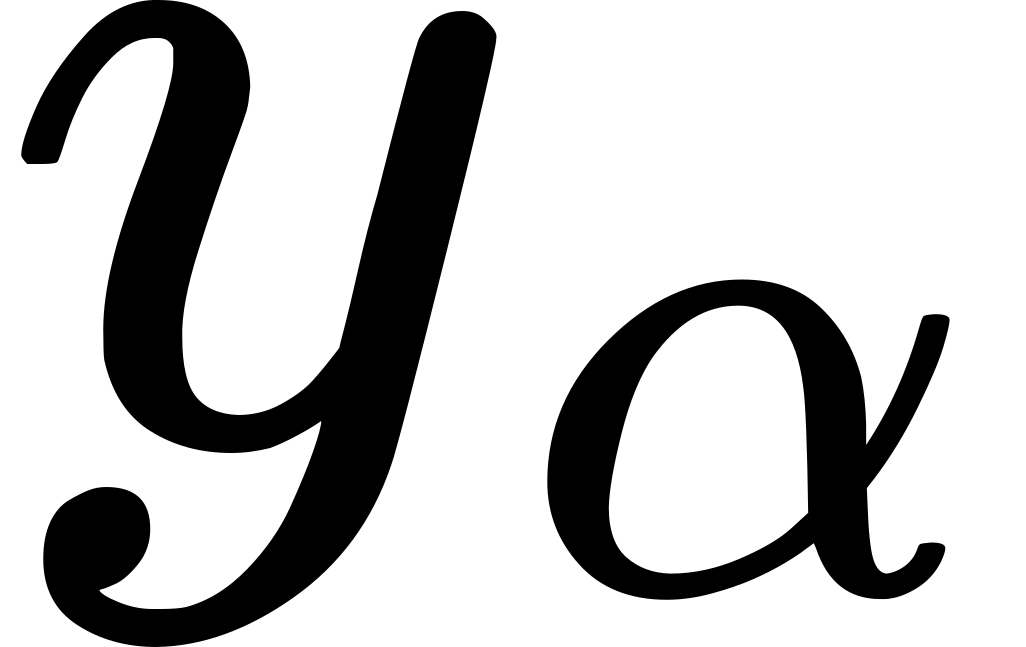
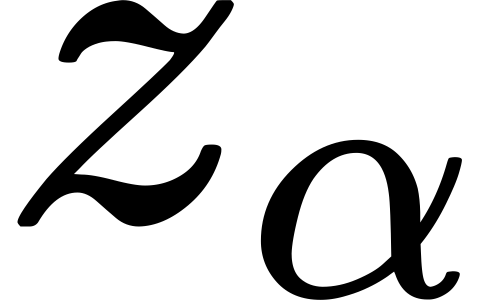
[where 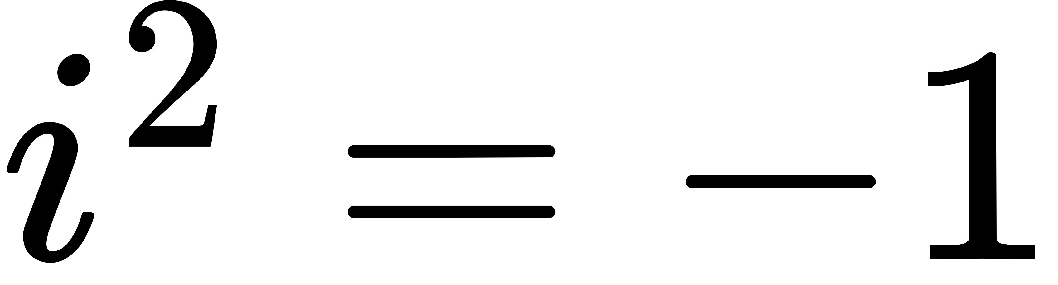 ]
| |
, |
 , |
 , |
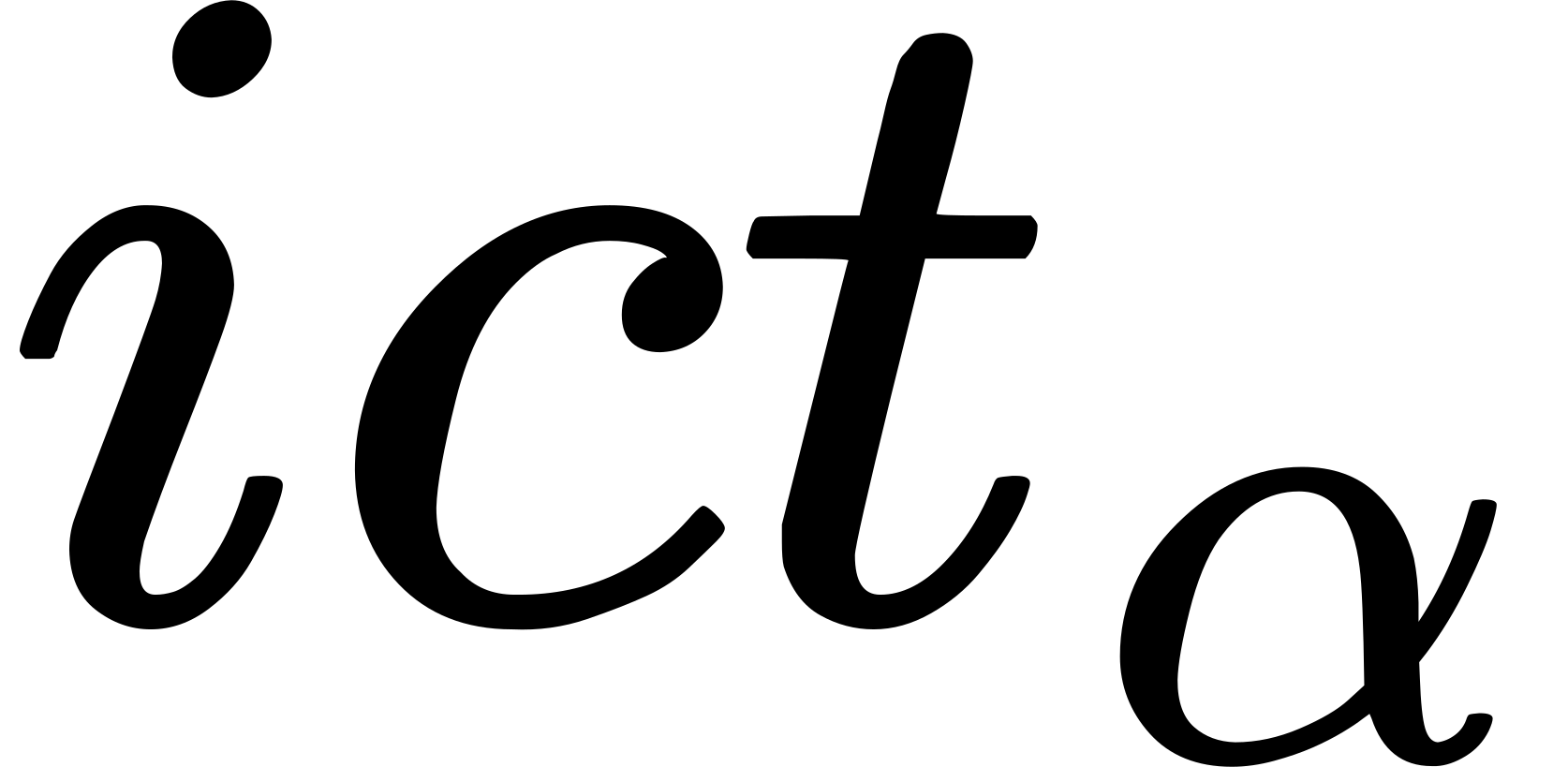 |
|
, |
0, |
0, |
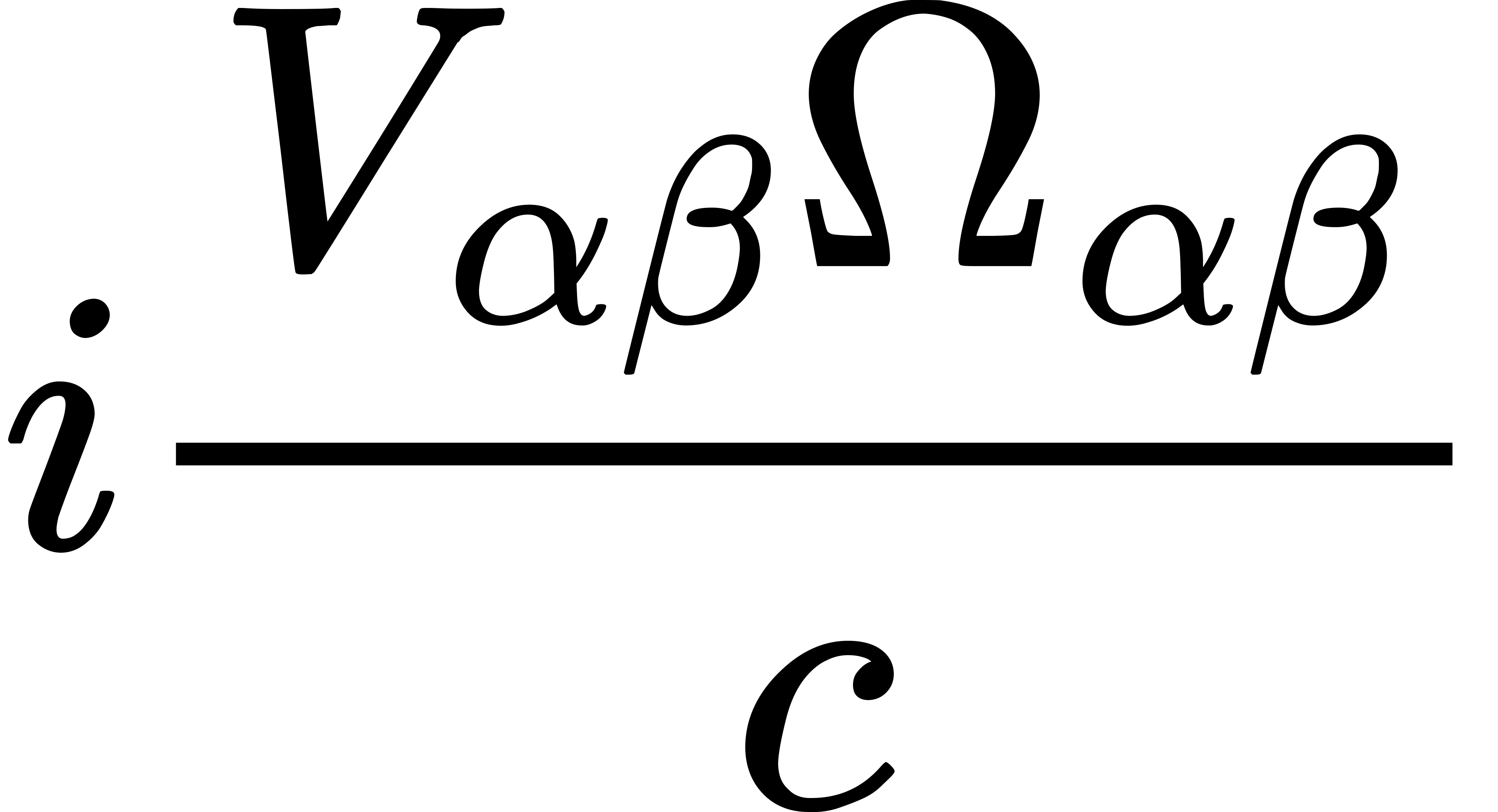 |
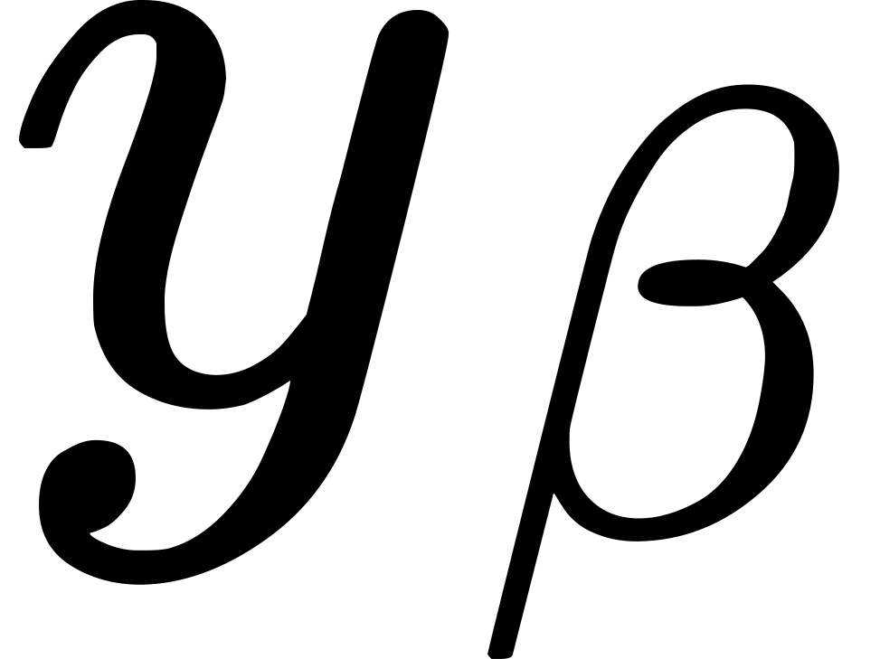 |
0, |
1, |
0, |
0 |
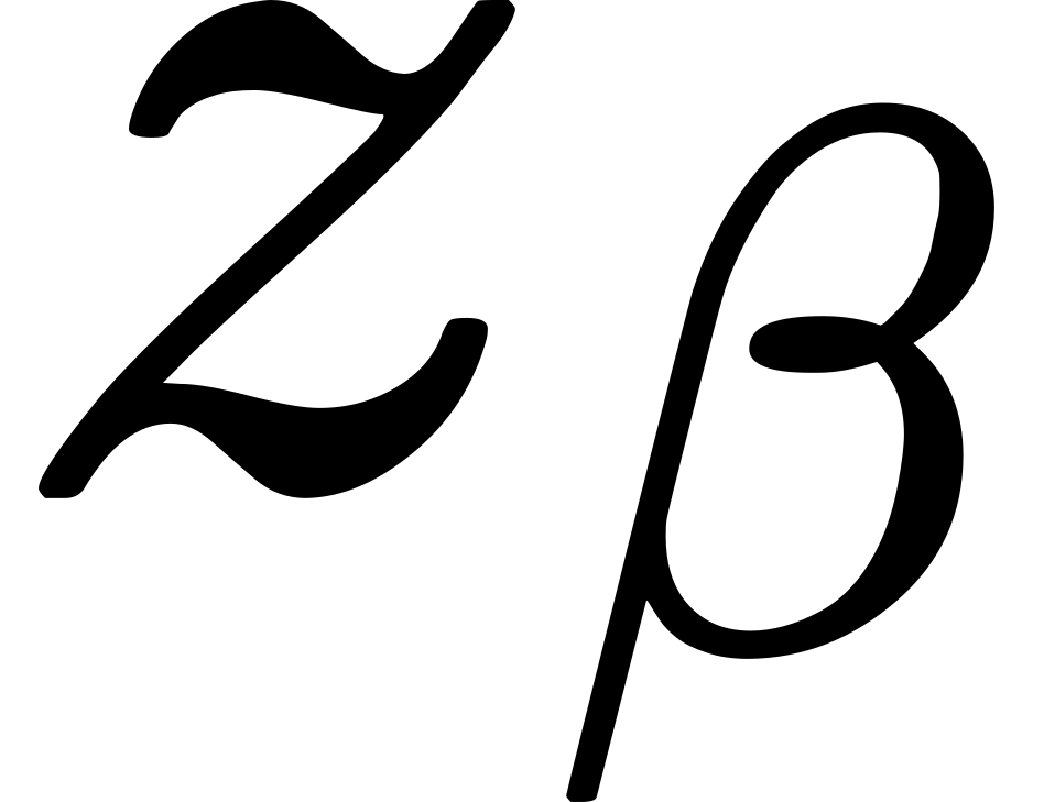 |
0, |
0, |
1, |
0 |
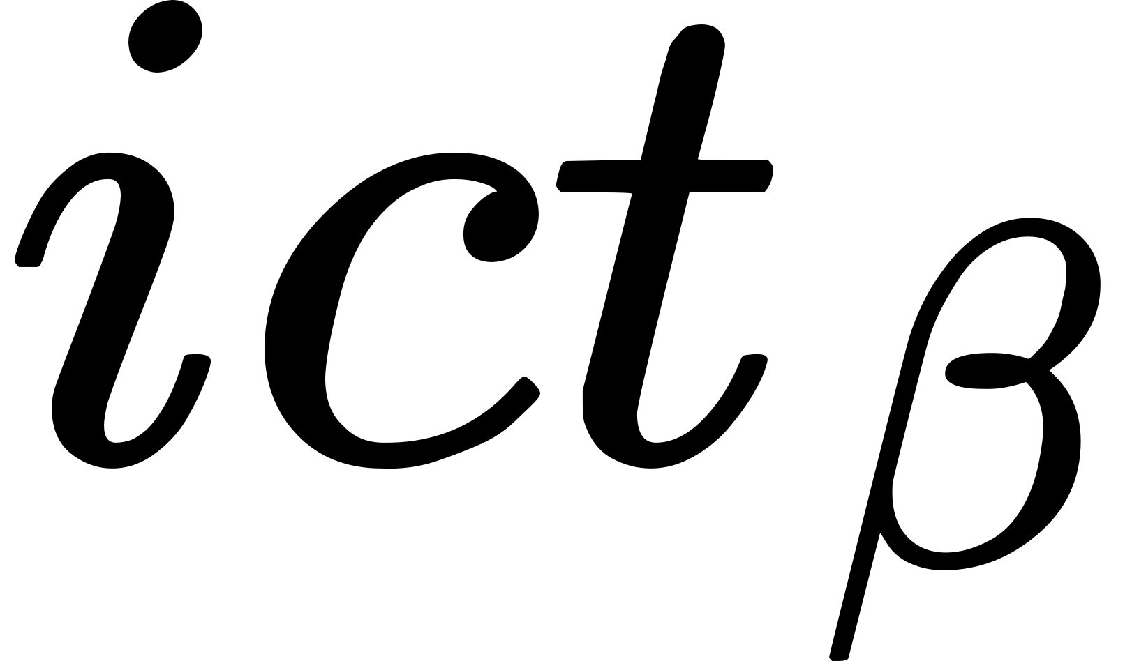 |
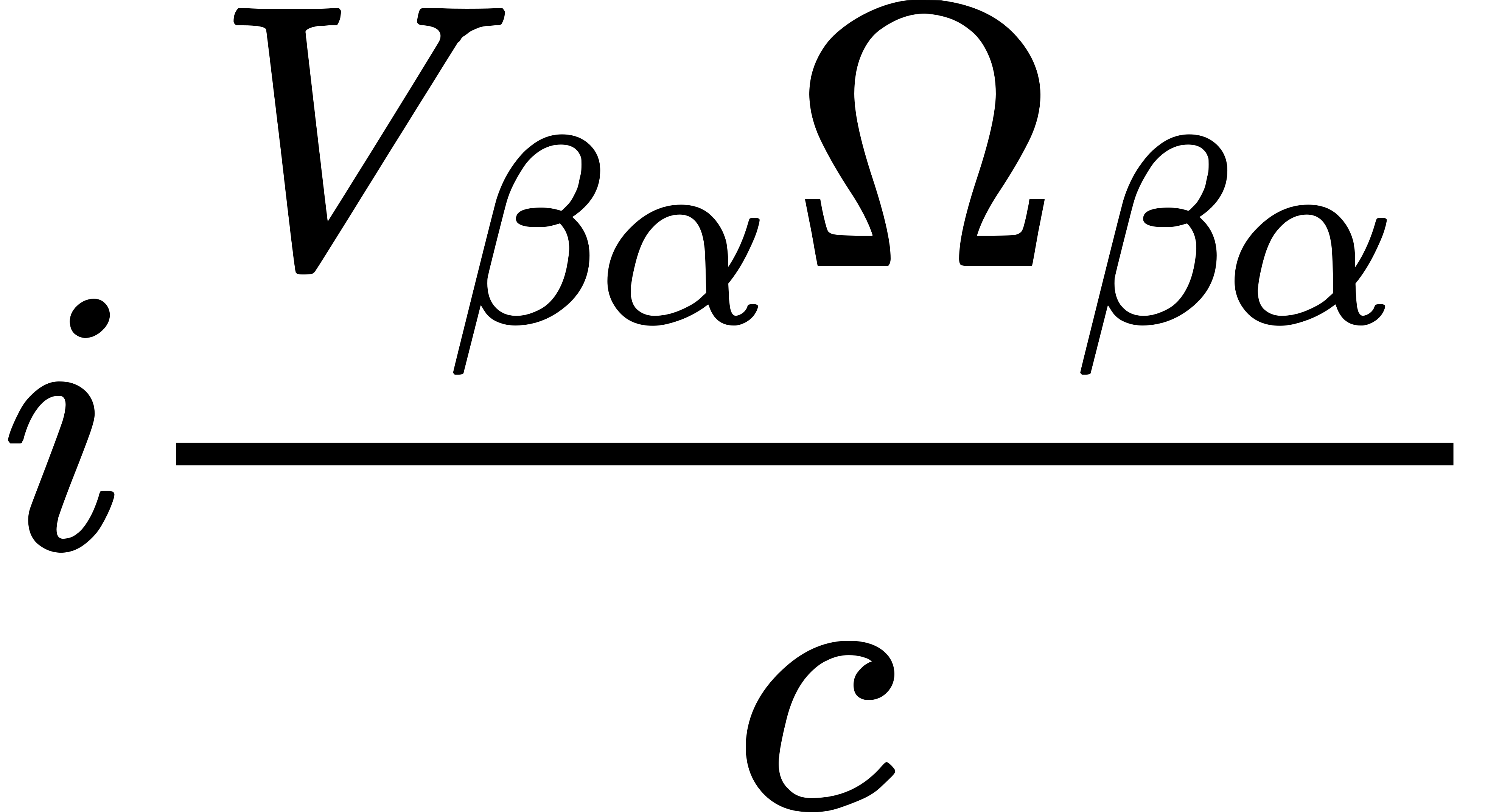 |
0, |
0, |
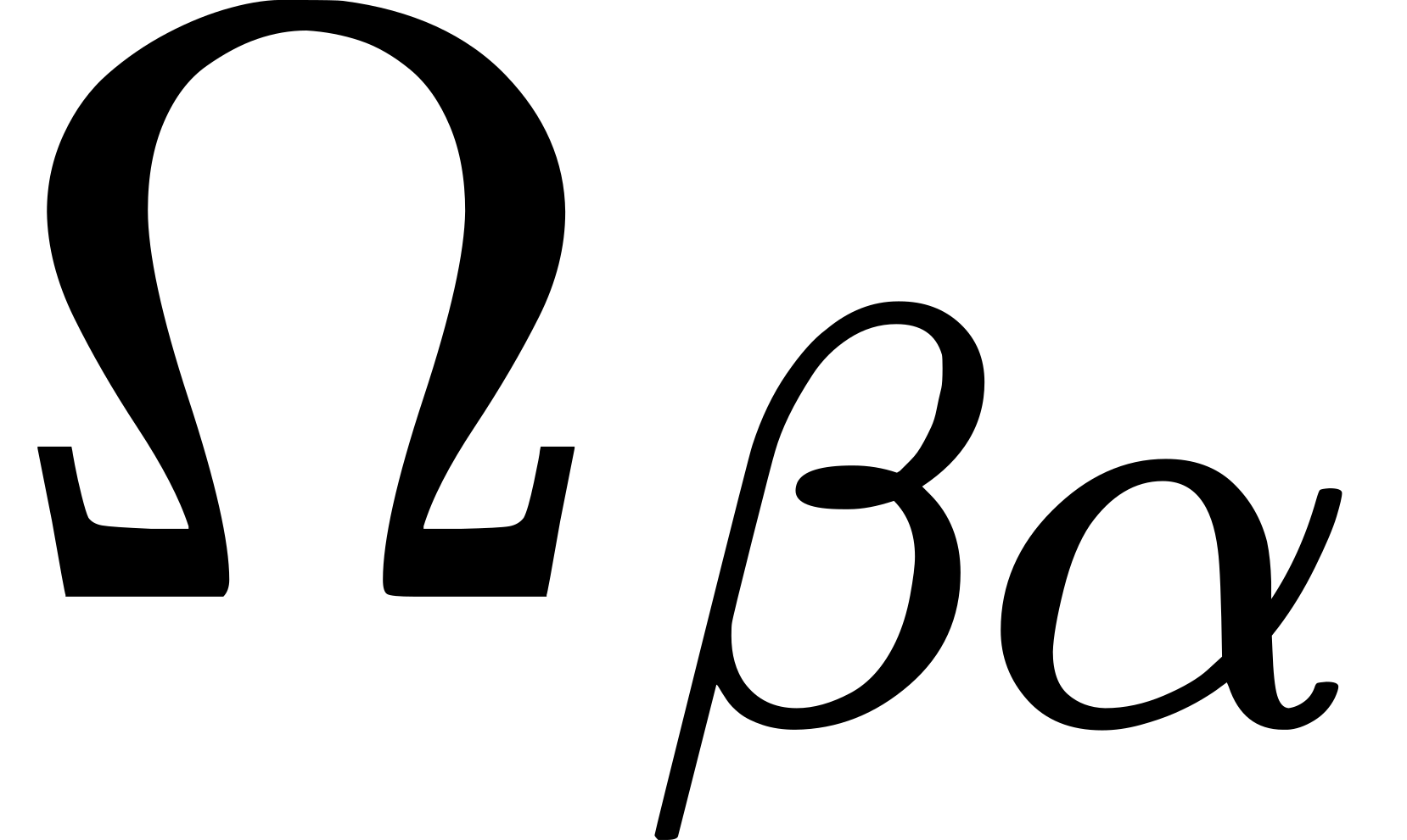 |
52.3 We notice that

The integral  taken throughout the four-dimensional region of the set of event-particles
which analyse [cf. 37.3] an event
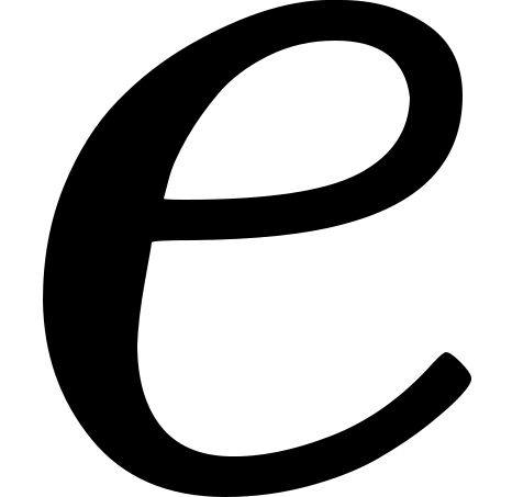 will be
called the 'absolute extent' of . It follows from (i) that the
absolute extent of an event is independent of the time-system in which
its measure is expressed.
Furthermore if be any function of
(), it can by (ii) of
52.2 be also expressed as a function of
(), and then by (i)
 or, in more familiar form,
 where the limits are taken to include some event.
We may expect important physical properties to be expressible in terms
of such integrals, in particular where is an invariant form for
the equations of transformation of 52.2, and when
the conditions, which the quantity represented by the integral
satisfies, are also invariant in their expression in different
time-systems.
The formulae of this subarticle hold of each type of kinematics.
52.4 The hyperbolic type of kinematics has issued in the formulae
of the Larmor-Lorentz-Einstein theory of electromagnetic relativity,
namely, the theory by which with a certain amount of interpretation the
electromagnetic equations are invariant for these transformations.
The physical meaning of  is also well known; namely, any velocity
which in any time-system is of magnitude is of the same magnitude
in every other time-system. No assumption of the existence of a velocity
with this property or of the electromagnetic invariance has entered into
the deduction of the kinematic equations of the hyperbolic type. A
velocity greater than cannot represent any time-system, and
accordingly its physical significance must be entirely different from
that of a velocity less than .
52.5 It is easily proved from (ii) of 52.2
that

If the origin and the event-particle , i.e.
(),
be co-momental and be the time-system whose moment , contains
, then by (i)

If and be sequent and on a point-track, and be
the time-system whose point 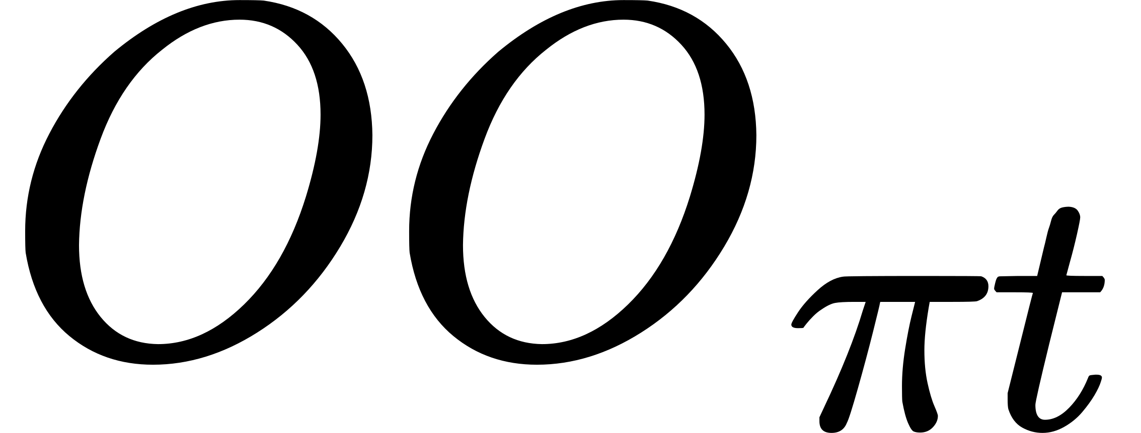 is occupied by ,
then by (i)

Thus there are three ways in which the 'separation' between two
event-particles ( and ) can be estimated; namely, (1) in any
assumed time-system the -distance between the
-points occupied by the event-particles measures
-space separation: (2) the lapse of -time between
the -moments occupied by the event-particles measures
-time separation: and (3) if the event-particles be co-momental,
 measures the 'proper' space separation and there is no 'proper' time
separation; and if the particles be sequent,
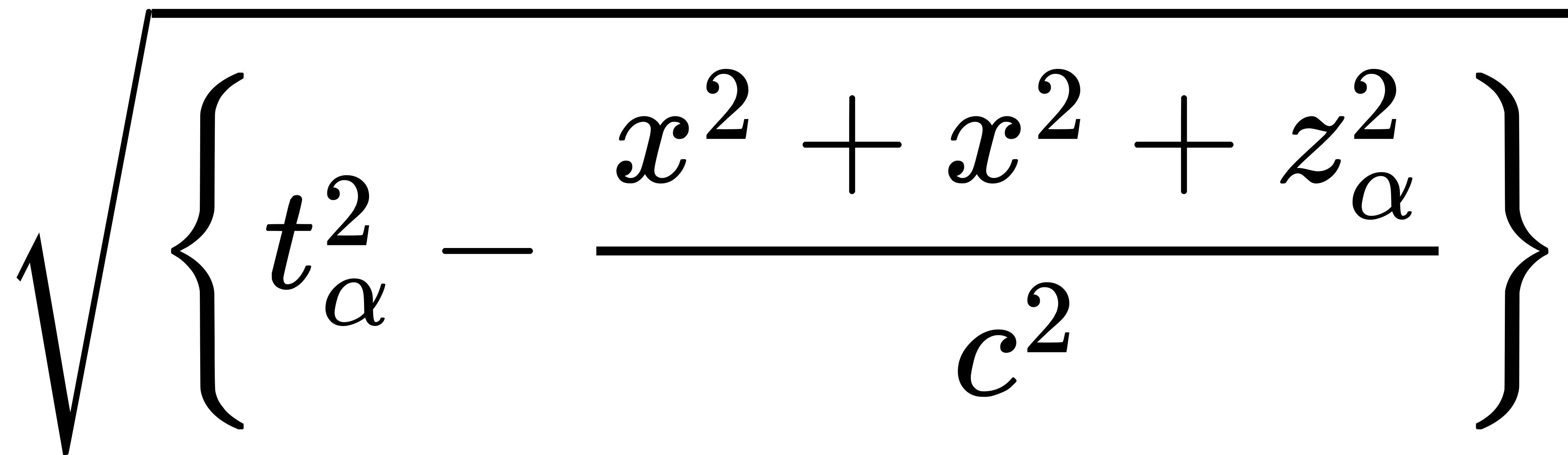 measures the 'proper' time separation and there is no
'proper' space separation.
In the framing of physical laws it is essential to consider what measure
of separation is relevant. It is to be noted that there may be
time-systems (other than ) of special relevance to the
phenomena in question. It is not at all obvious that invariance of form
in respect to all time-systems is a requisite in the complete expression
of such laws; namely, the demand for relativistic equations is only of
limited applicability.
If and be on a null-track

Event-particles on the same null-track may be expected to have special
physical relations to each other. Call such event-particles 'co-null.'
52.6 We may conceive a special time-system
associated (by some means) with each event-particle
(). Thus is a
function of these four co-ordinates of a particle; or in other words,
(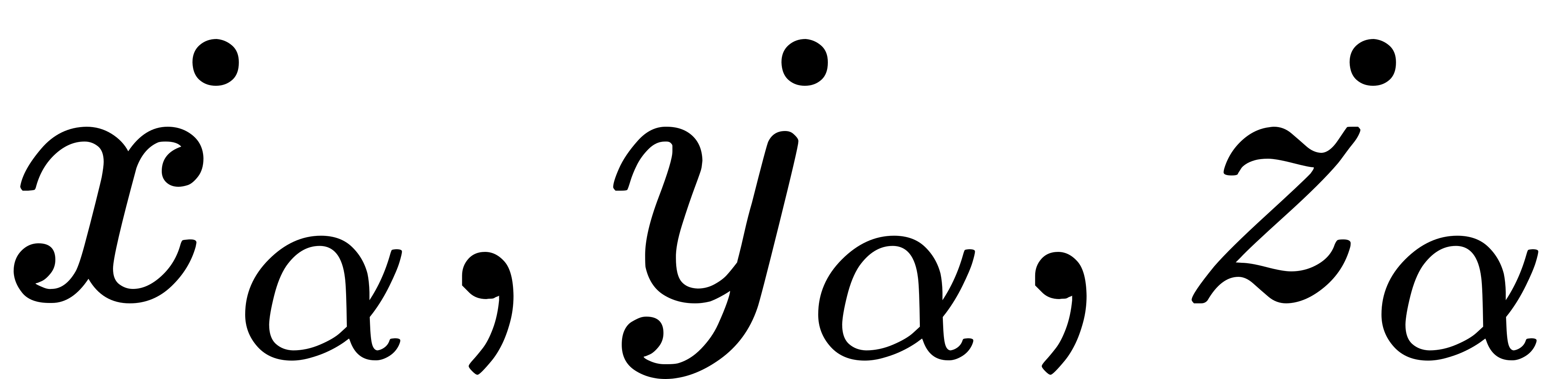 )
are functions of ().
A correlation of time-systems to event-particles which is one-many, so
that there is one and only one time-system corresponding to each
event-particle, is called a 'complete kinematic correlation.' The
portion of that correlation which only concerns event-particles at the
time is called a 'kinematic -correlation.'
Other portions can be selected by confining the event-particles to
certain regions in the -space.
If in a certain kinematic correlation the time-system it be correlated to
(), then is
called the time-system of
() 'proper' to that
correlation. The 'proper' time-system of an event-particle always
refers to a certain kinematic correlation implicitly understood.
Furthermore ()
is the velocity at () due to the
implicitly understood kinematic correlation at the -time
.
Then, being the proper time-system at
(),

Then equations (iii) of 52.2 can be written

The kinematic symmetry as between and is now
apparent in the formulae. The first of equations (ii) can be replaced by

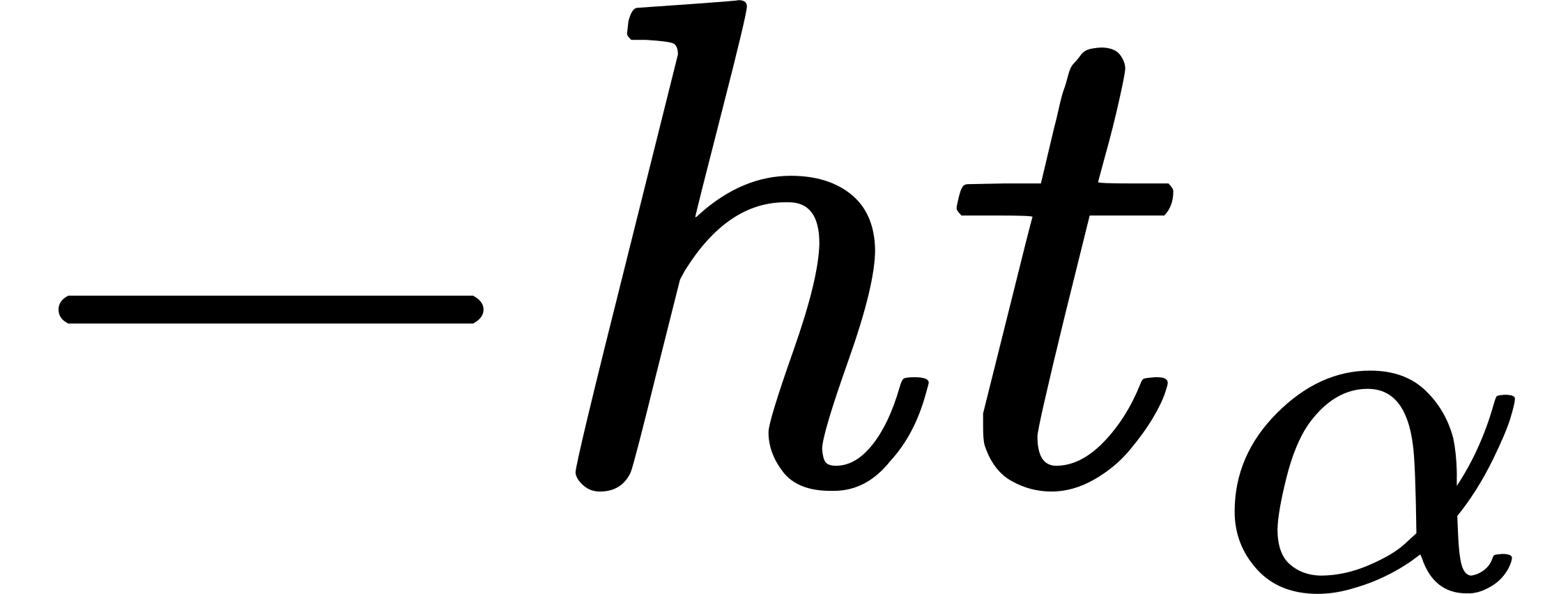
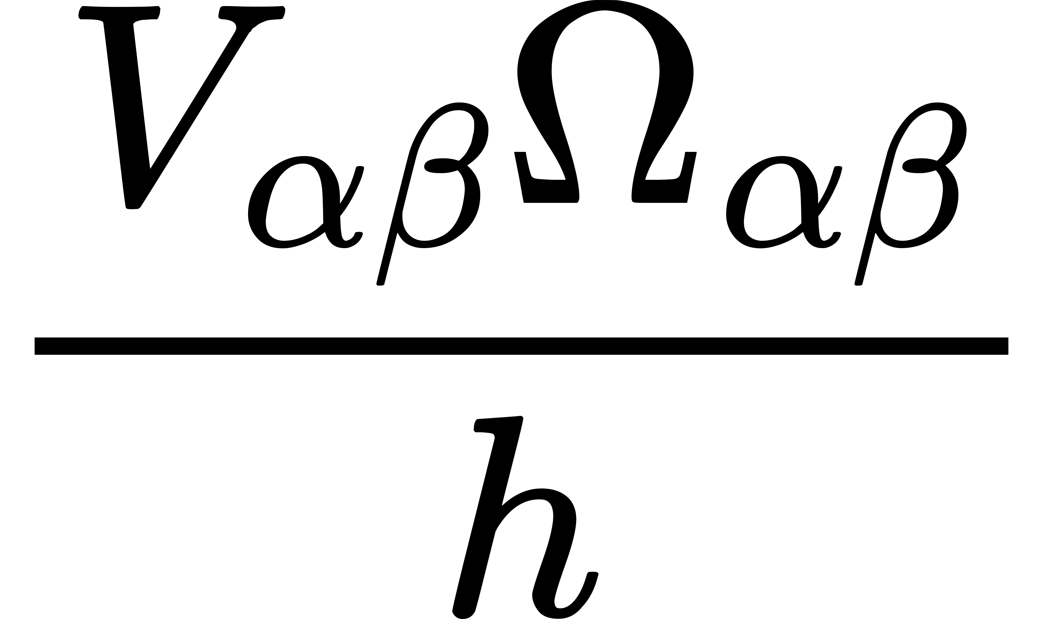
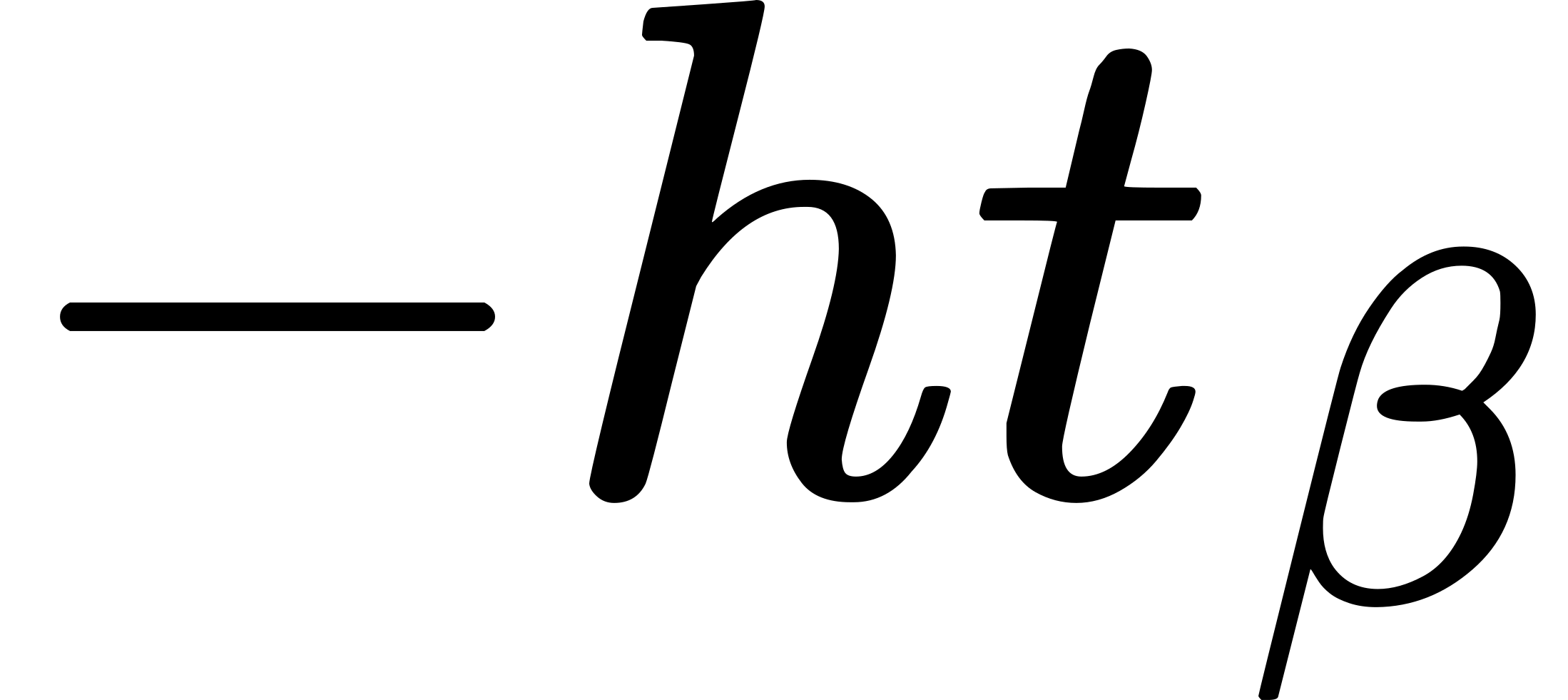
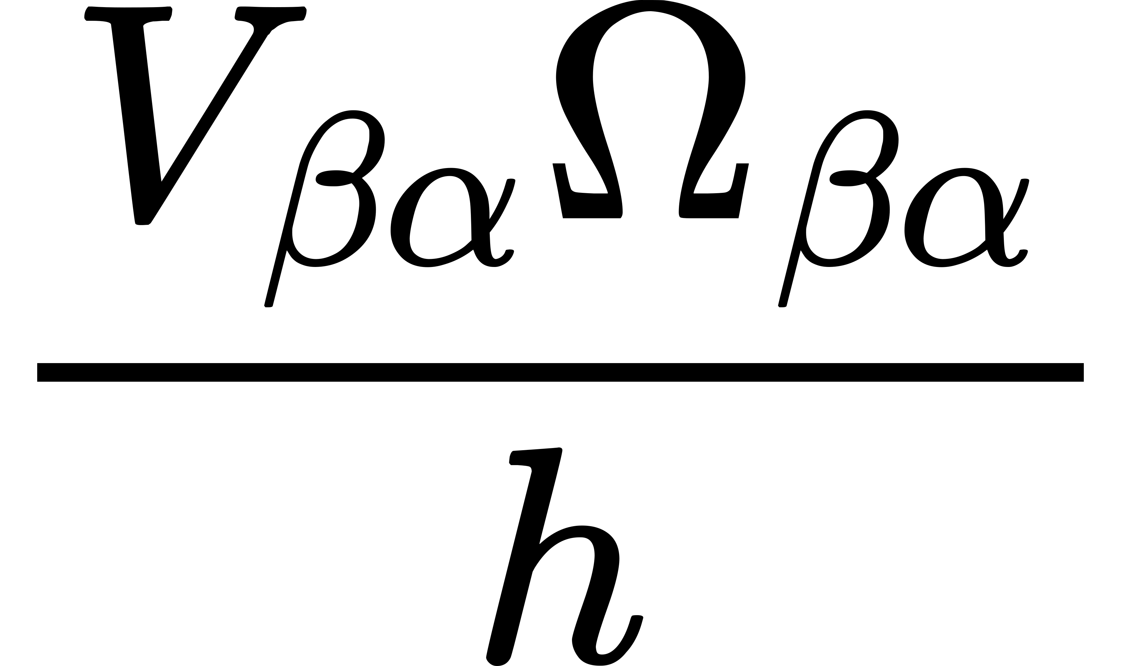
52.7 In considering the elliptic type of kinematics put 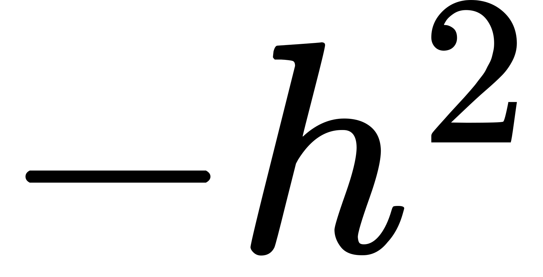 for . The equations of article 51 are now
embodied in the scheme
| |
, |
, |
, |
 |
|
, |
0, |
0, |
 |
|
0, |
1, |
0, |
0 |
|
0, |
0, |
1, |
0 |
 |
 |
0, |
0, |
|

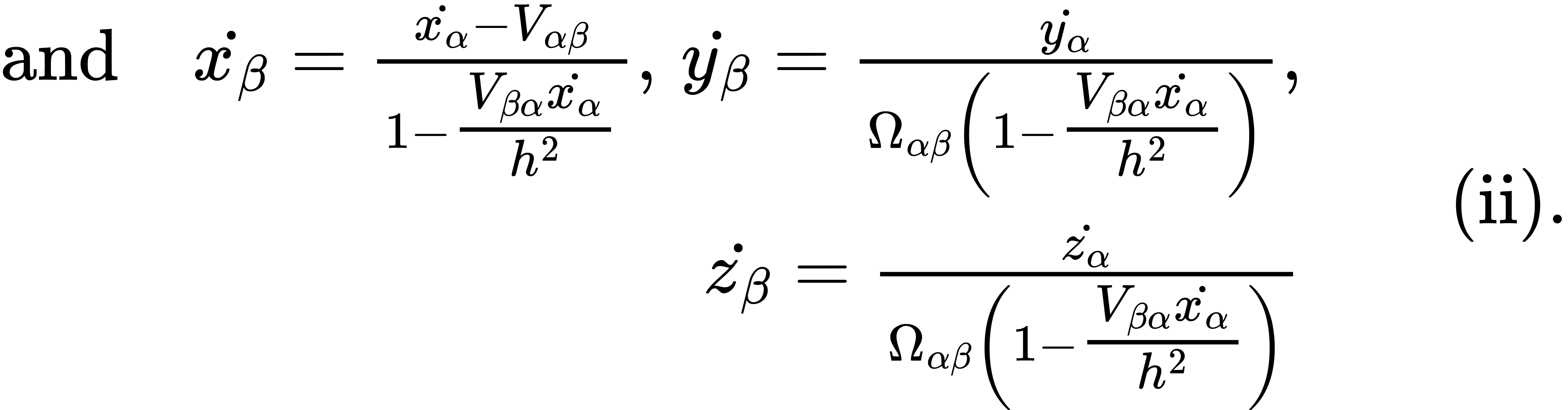

The fundamental distinction between space and time, i.e. between rects
and point-tracks, has failed to find any expression in the formulae for
measurement relations. Accordingly with this type of kinematics, it
would be natural to suppose that the distinction does not exist and that
every rect was a point-track and every point-track a rect. This
conception is logically possible but does not appear to correspond to
the properties of the external world of events as we know it.
Furthermore the electromagnetic equations lose their invariant property.
Altogether there appear to be good reasons for putting aside the
elliptic type of kinematics as inapplicable to nature.
52.8 In the parabolic type of kinematics we put 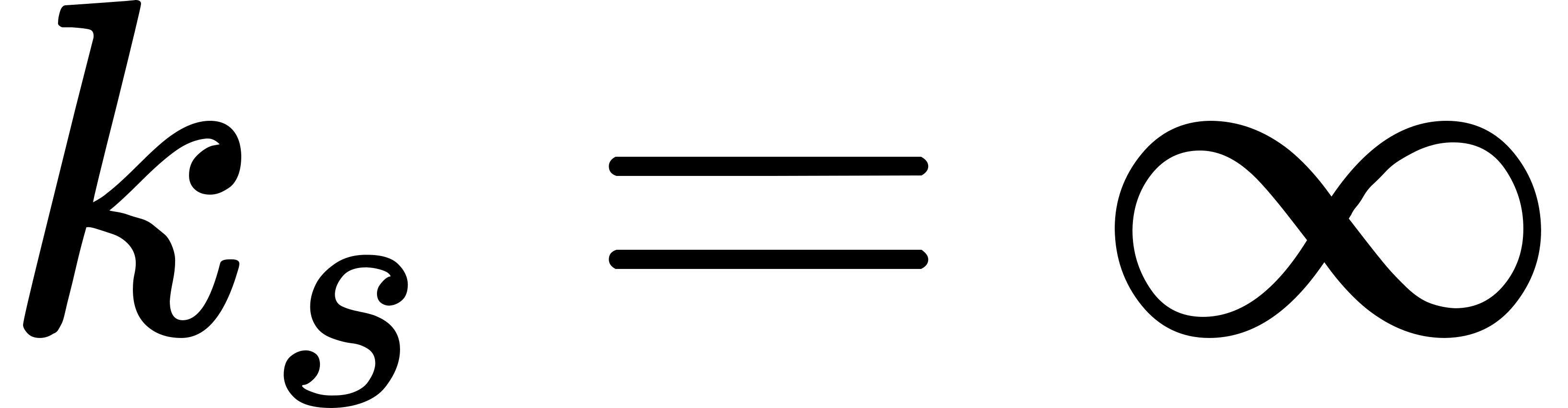 Hence

Then from (ii) of 51.1 and (ii) of
50.3 and (iii) of 50.1

Thus equations (i) of 49.7 give

These are the formulae for the ordinary Newtonian relativity.
These formulae are well in accordance with common sense and are in fact
the formulae naturally suggested by ordinary experience. To some extent
the hyperbolic formulae lead to unexpected results, though, if be
a velocity not less than that of light, the divergences from the
deliverances of common sense take place in respect to phenomena which
are not manifest in ordinary experience. But when by refined methods of
observation the divergences between the two types of kinematics should
be apparent to the senses, experiment has, so far, pronounced in favour
of the hyperbolic type. Accordingly it is this type which we consider in
the sequel.
52.9 There is however one objection to the hyperbolic type, as
compared to the parabolic type, which is worth considering. In the
hyperbolic kinematics there is an absolute velocity with special
properties in nature. The difficulty which is thus occasioned is rather
an offence to philosophic instincts than a logical puzzle. But certainly
our familiar experience, in some way which it is difficult to formulate
in words, leads us to shun the introduction of such absolute physical
quantities. This particular difficulty is largely diminished by noting
that the existence of with its peculiar properties really means
that the space-units and time-units are comparable; namely, there is a
natural relation between them to be expressed by taking to be
unity. Either the time-unit would then be inconveniently small or the
space-unit inconveniently large; but this inconvenience does not alter
the fact that congruence between time and space is definable. Always
when a possible definition of congruence is omitted, such absolute
physical quantities occur. The fact that, so far as time and space are
concerned, the existence of a congruence theory seems paradoxical is due
to absence of any phenomena depending on that theory except in very
exceptional circumstances produced by refined observations.
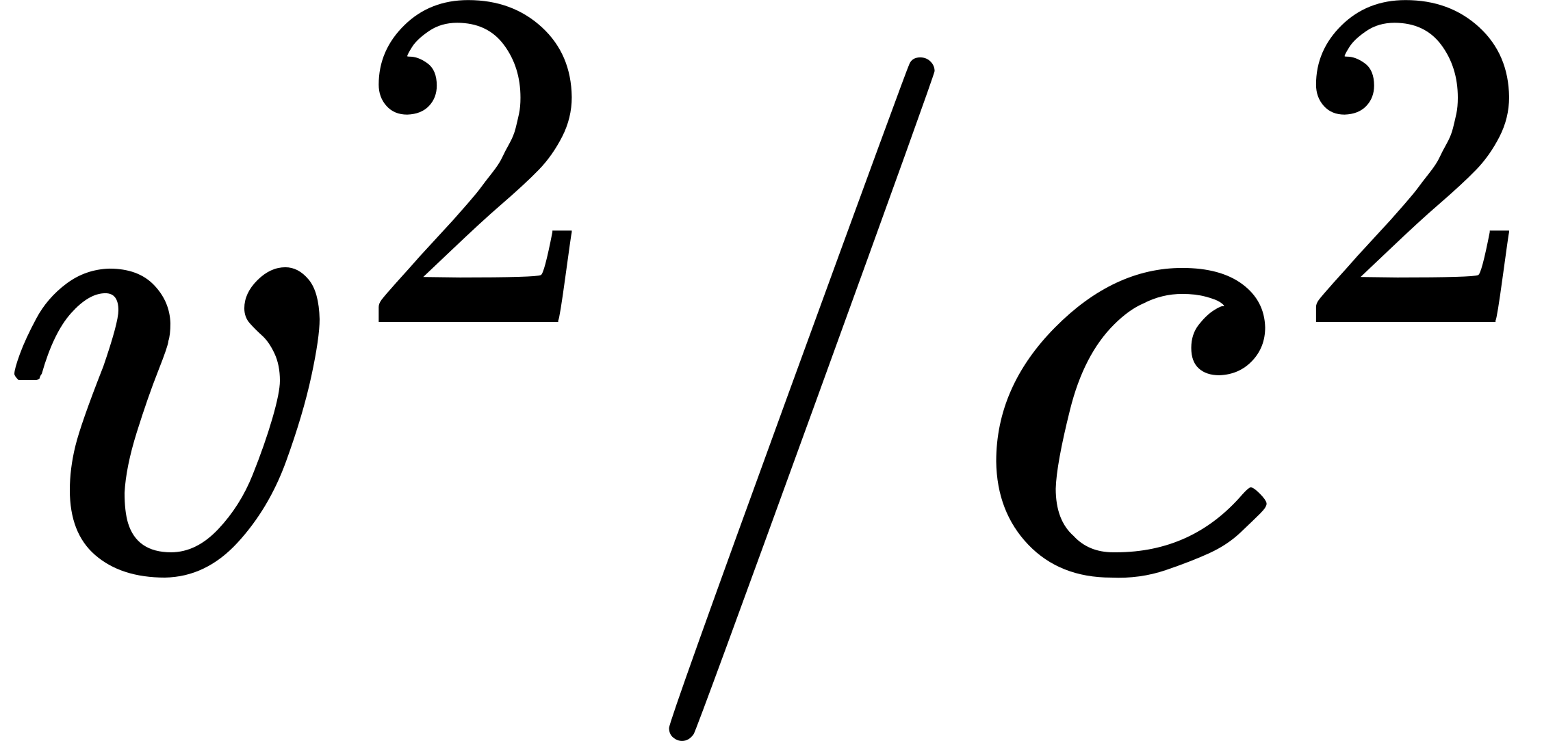 of the main effect [
 being the velocity of
the matter and
 and
 is the fact that their states of change are partly dependent on
their relative locations and natures. The disconnection involved in
spatial separation leads to reduction of such causal action to the
transmission of stress across the bounding surface of contiguous
materials. But what is contact? No two points are in contact. Thus the
stress across a surface necessarily acts on some bulk of the material
enclosed inside. To say that the stress acts on the immediately
contiguous material is to assert infinitely small volumes. But there are
no such things, only smaller and smaller volumes. Yet (with this point
of view) it cannot be meant that the surface acts on the interior.
 with
 , as well as such relations between

 ),
(
 )
and (
 ), namely the electric and
magnetic 'forces' and the velocity of the charge of electricity. Now a
vector involves direction; and direction is not concerned with what is
merely at that point. It is impossible to define direction without
reference to the rest of space; namely, it involves some relation to the
whole of space.
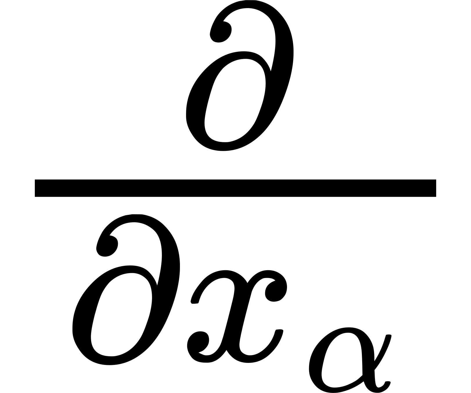 ,
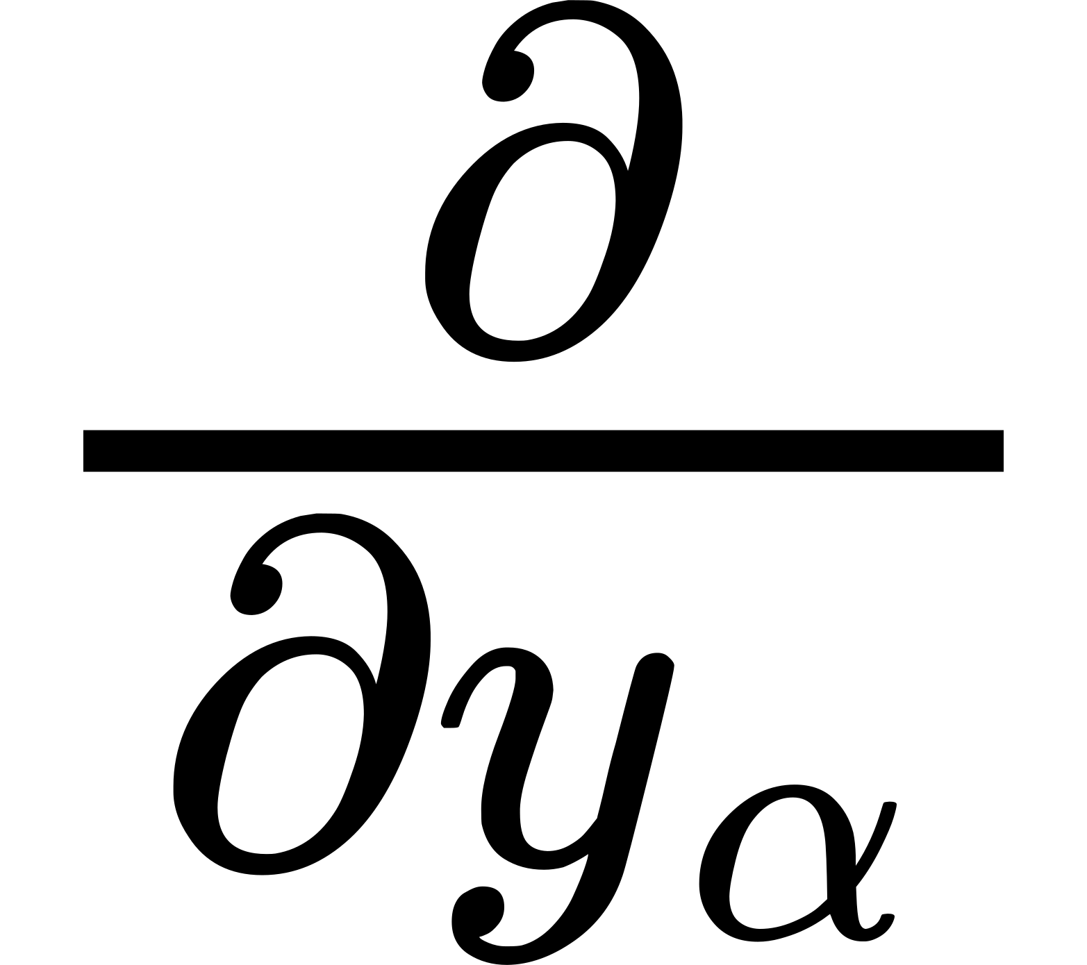 ,
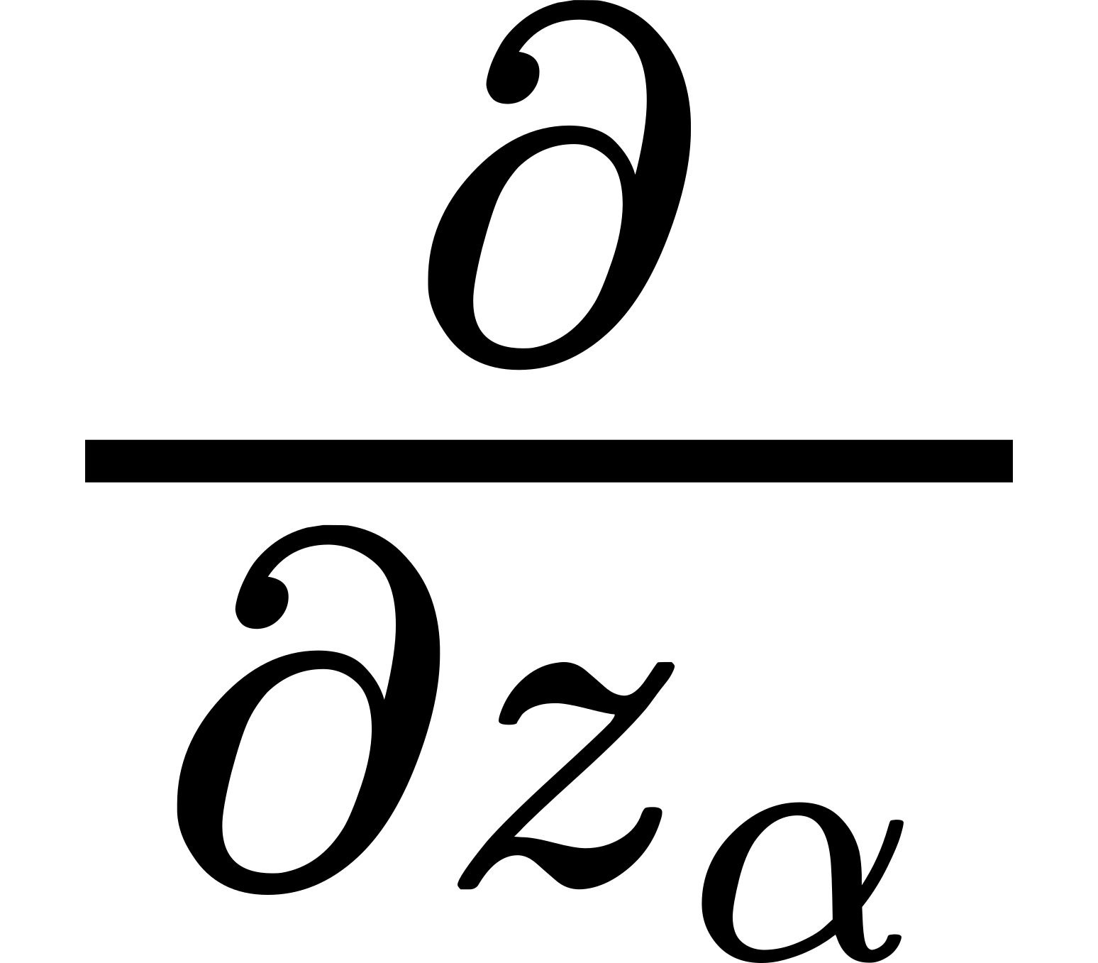 , which enter through the symbols
 ; and
they also involve the temporal differential operator
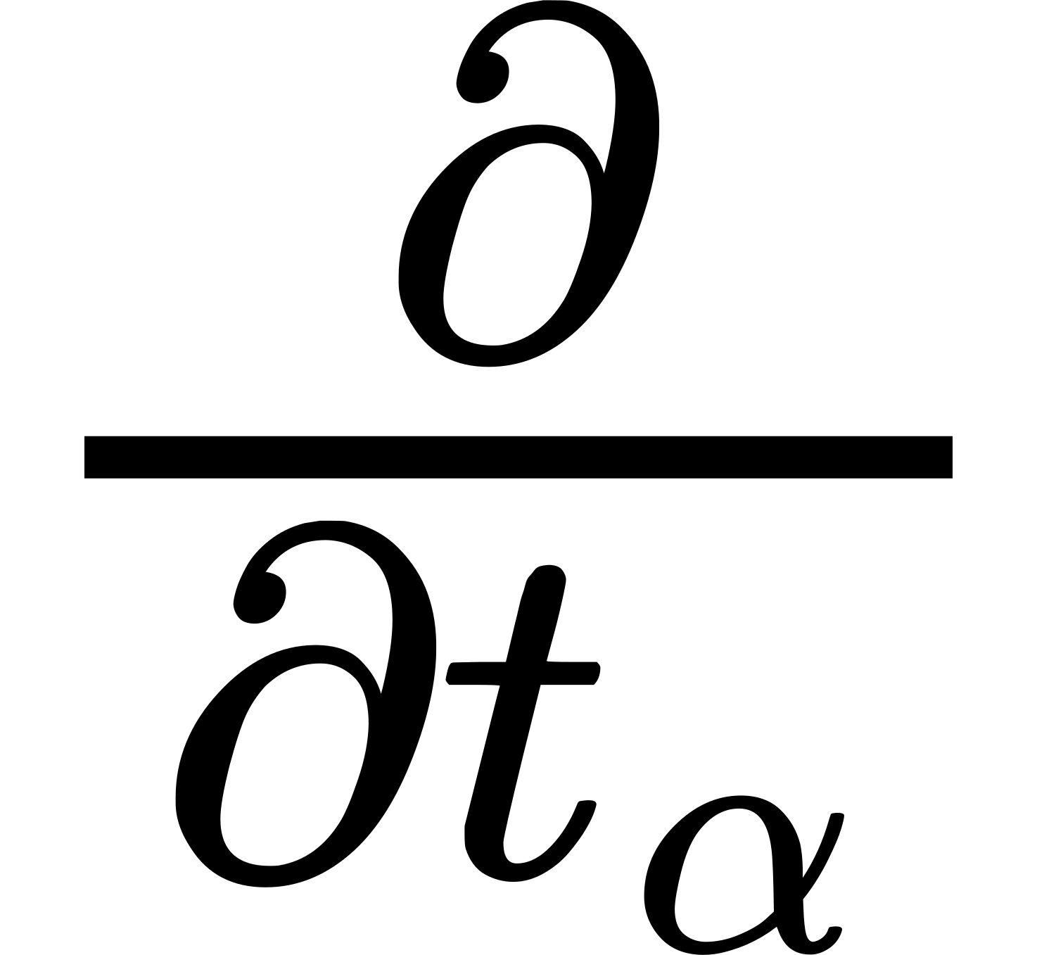 . The
differential coefficients thus produced essentially express properties
in the neighbourhood of the point (
 and
 )
express properties. Such an ether has certainly a very
shadowy existence; and yet we cannot assume that it moves, merely for
the sake of giving it something to do.
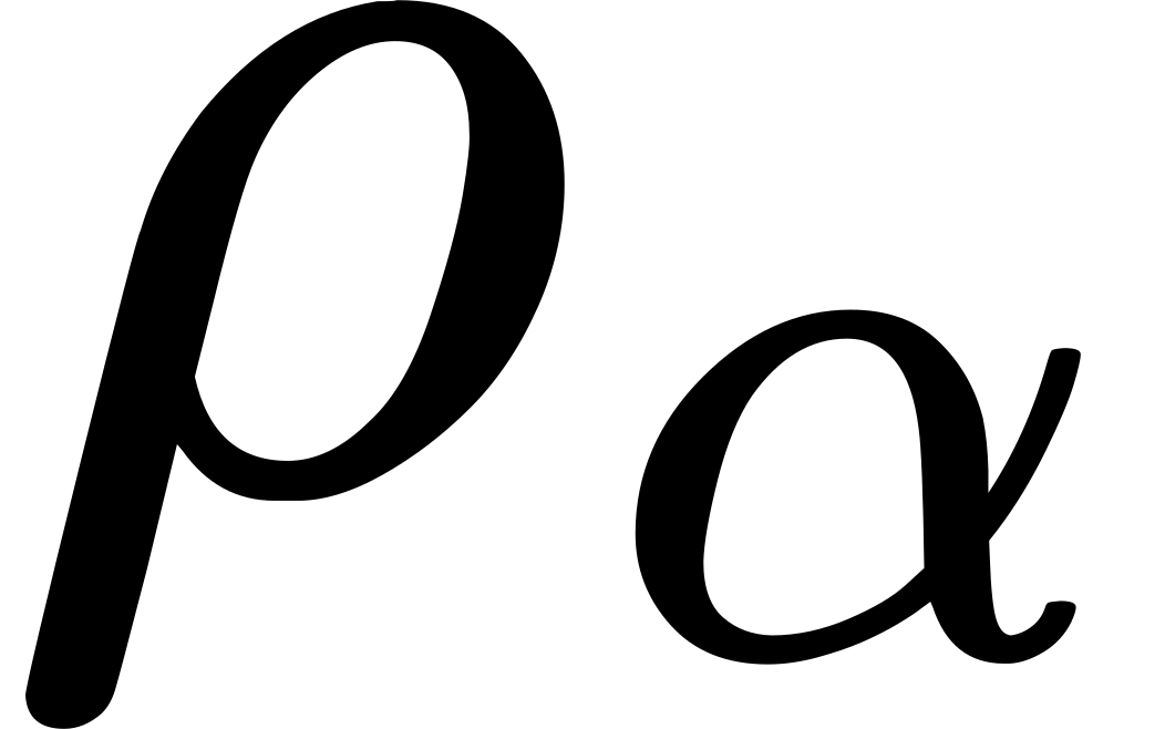 (the volume-density of the charge),
(
 ) and
(
 ).
But this is merely to say that the ultimate facts
contemplated by Maxwell's equations are certain events which are
occurring throughout all space. The material called ether is merely the
outcome of a metaphysical craving. The continuity of nature is the
continuity of events; and the doctrine of transmission should be
construed as a doctrine of the coextensiveness of events with space and
time and of their reciprocal interaction. In this sense an ether can be
admitted; but, in view of the existing implication of the term,
clearness is gained by a distinction of phraseology. We shall term the
traditional ether an 'ether of material' or a 'material ether,'
and shall employ the term 'ether of events' to express the
assumption of this enquiry, which may be loosely stated as being 'that
something is going on everywhere and always.' It is our purpose to
express accurately the relations between these events so far as they are
disclosed by our perceptual experience, and in particular to consider
those relations from which the essential concepts of Time, Space, and
persistent material are derived. Thus primarily we must not conceive of
events as in a given Time, a given Space, and consisting of changes in
given persistent material. Time, Space, and Material are adjuncts of
events. On the old theory of relativity, Time and Space are relations
between materials; on our theory they are relations between events.
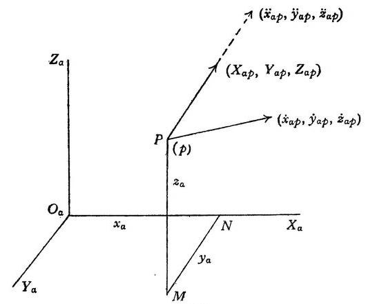
 ) as in the accompanying
figure be rectangular axes at rest; let
(
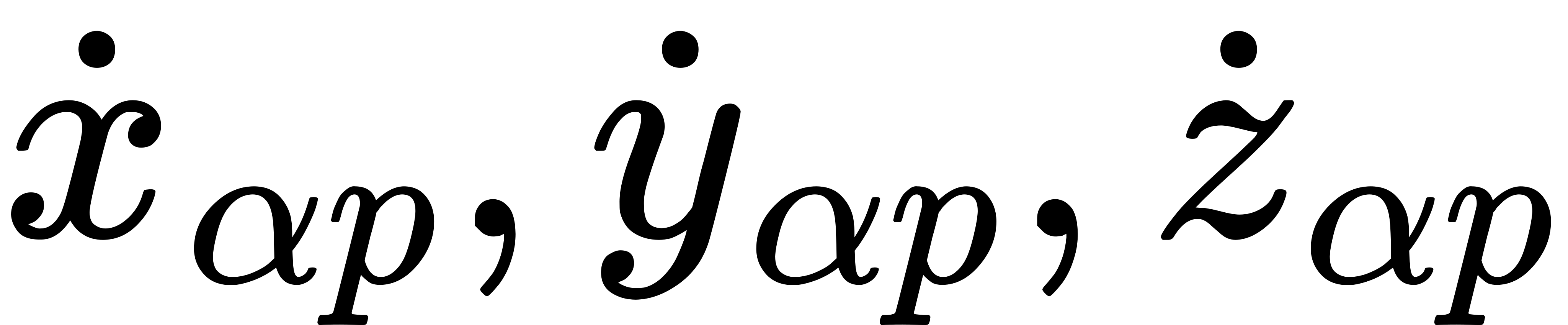 )
be the velocity of a material particle
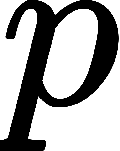 of mass
 ) relative to these axes, and let
(
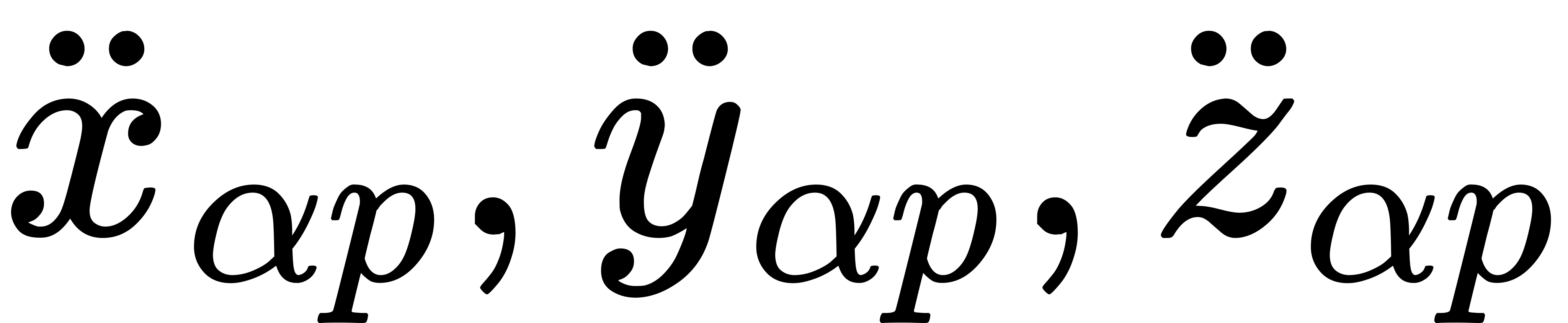 )
be the acceleration of the same particle. Also let
(
 ) be the force on the
particle

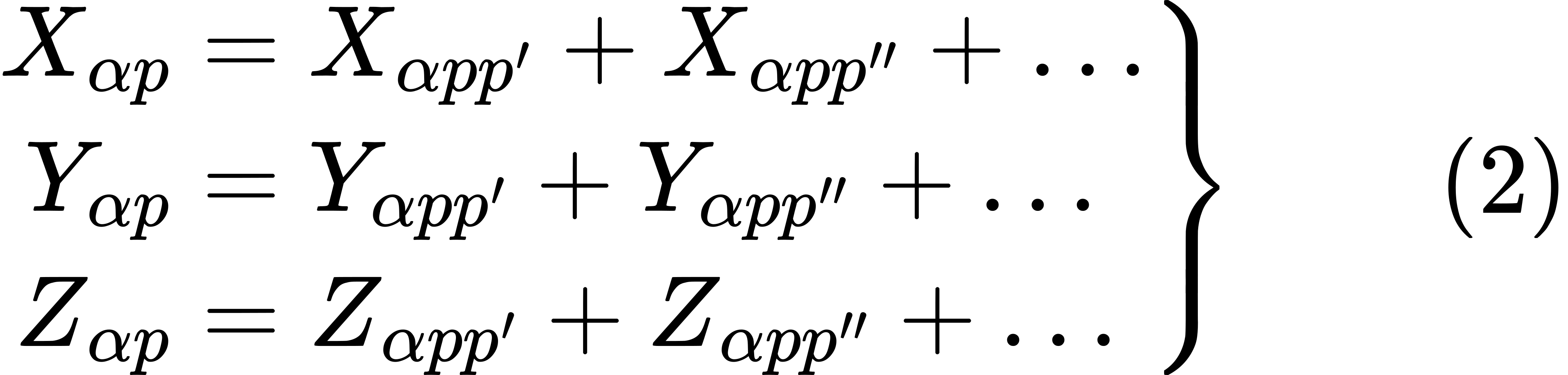
 ) is due to
 )
to
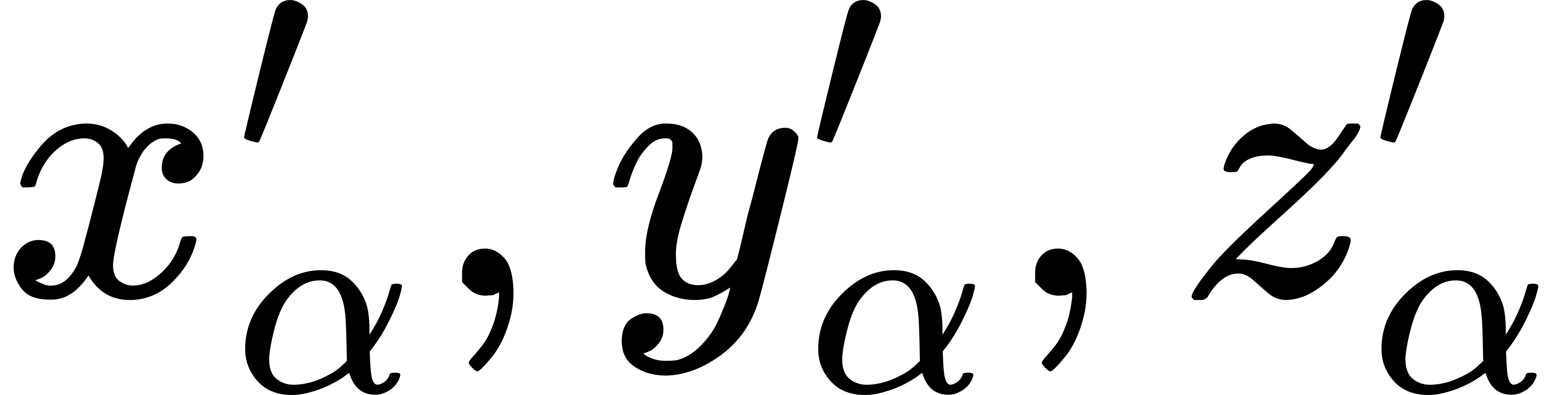 ) and
(
 )
be the acceleration of
 ) be
the force on
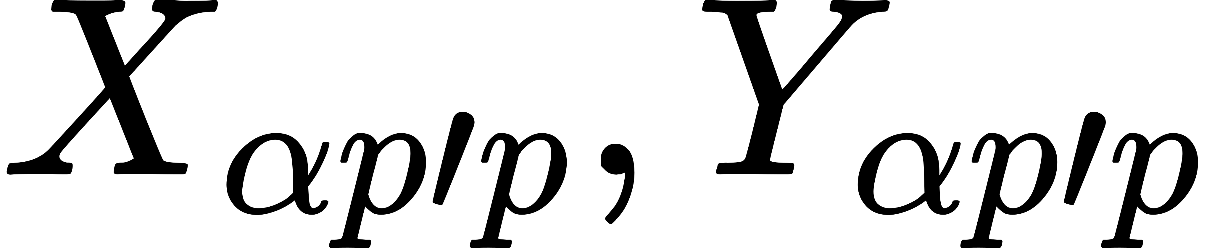 , etc.
have meanings for
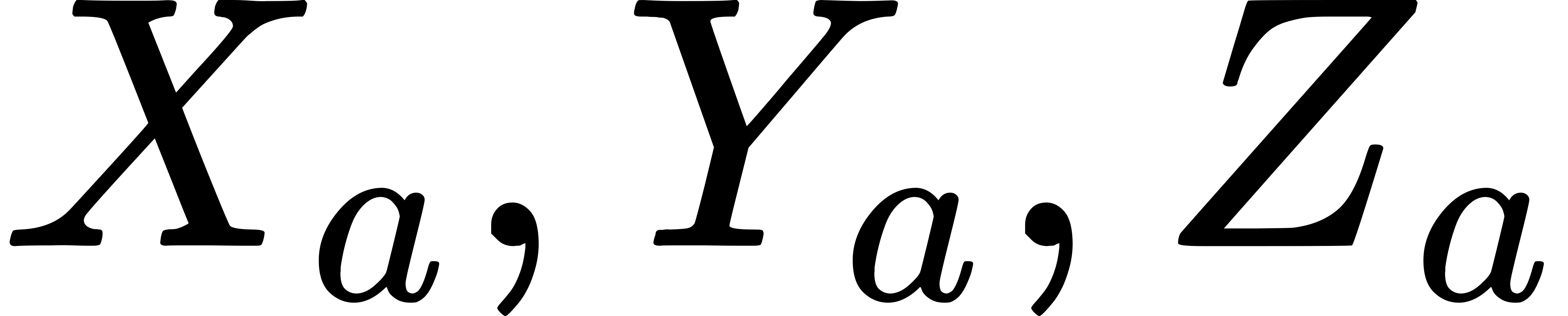
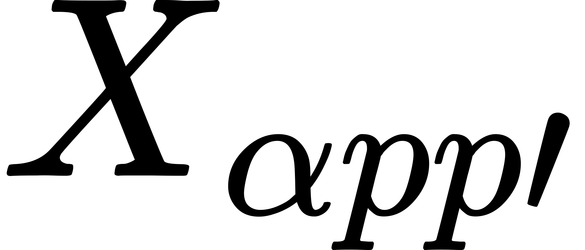 ,
etc. have for



 ) be any such vector. Then
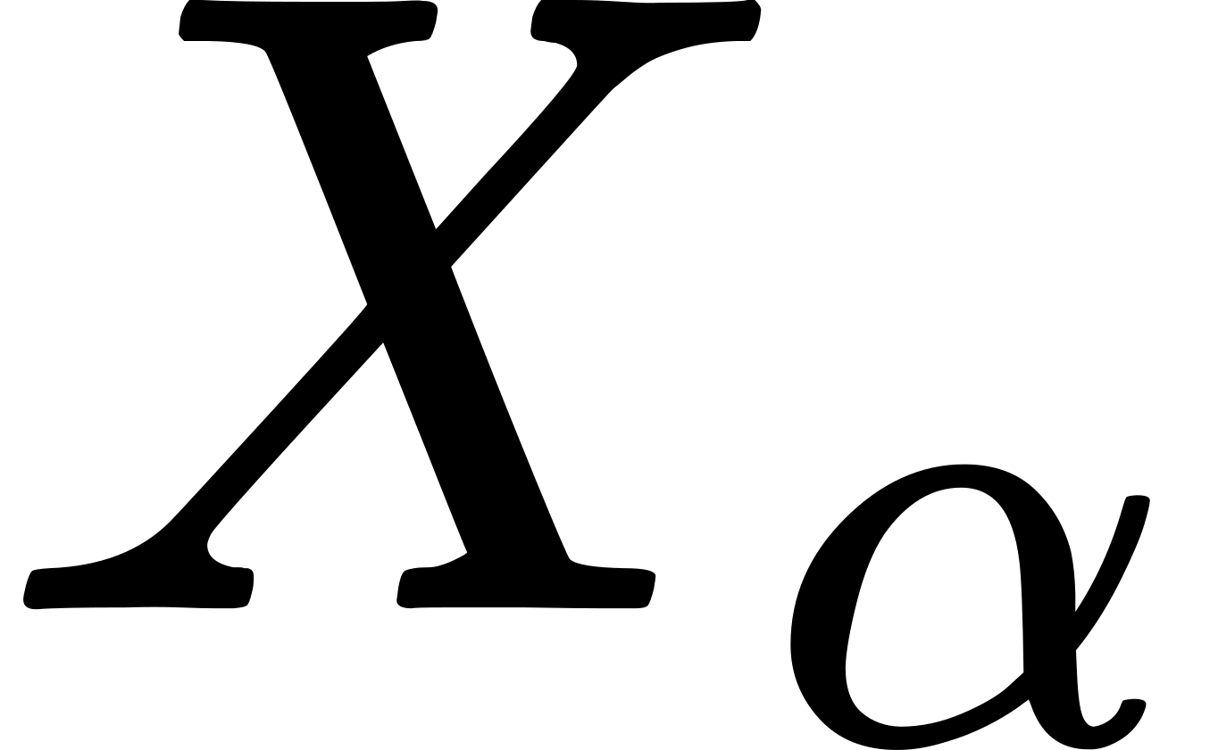 and
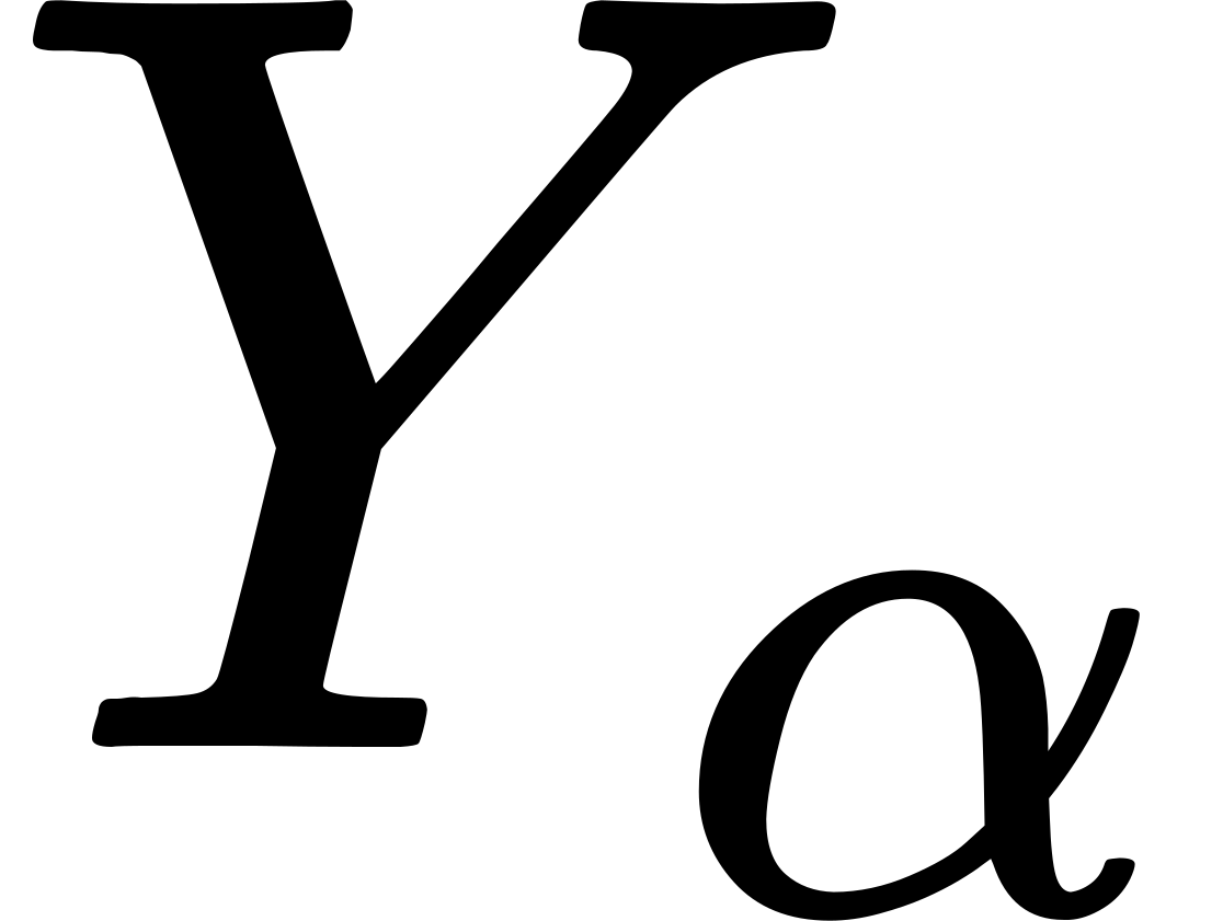 and
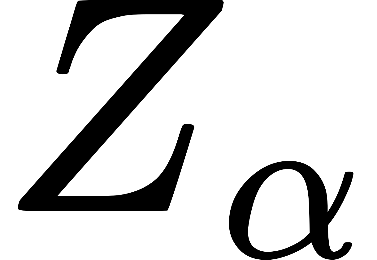 are each of them
functions of (
 . We shall assume that
our physical quantities are differentiable, except possibly at
exceptional points.
 ) stand for
(
 ), and analogously


 ) for the
vector

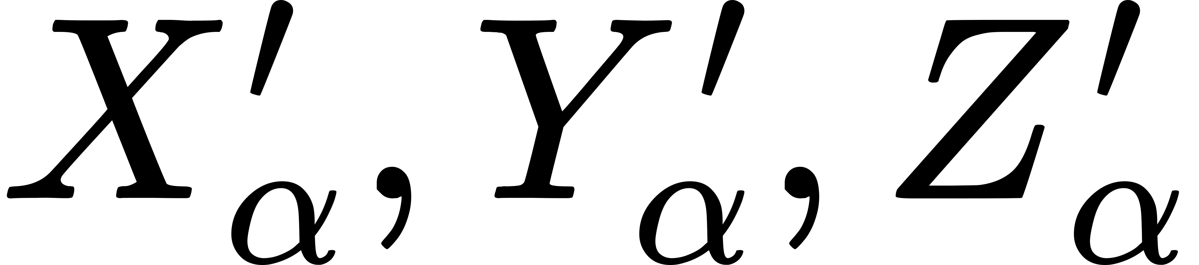 )
be another vector at the same point, then


 )
can be expressed in the symbolic form



 ) be the electric force at
 ), and let
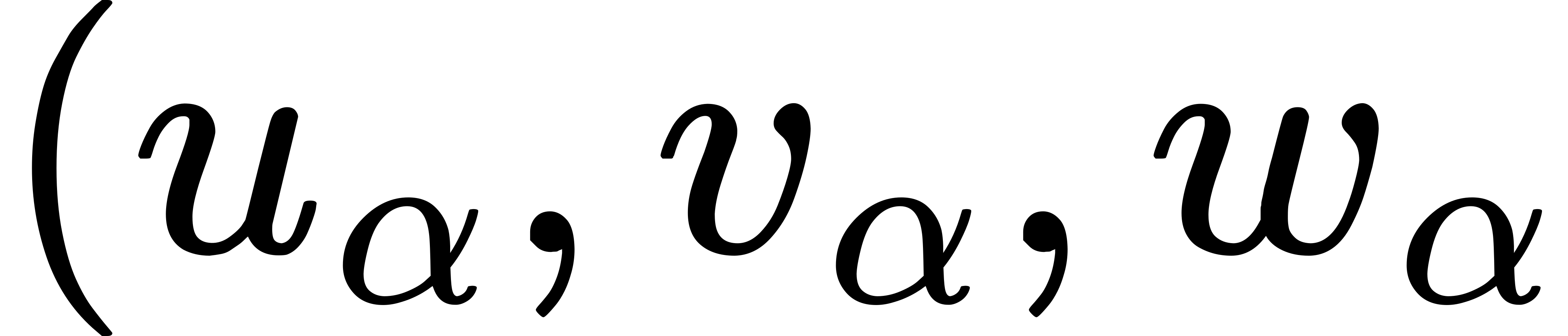 ) its
velocity; and let
 )
be the ponderomotive force: all equally at

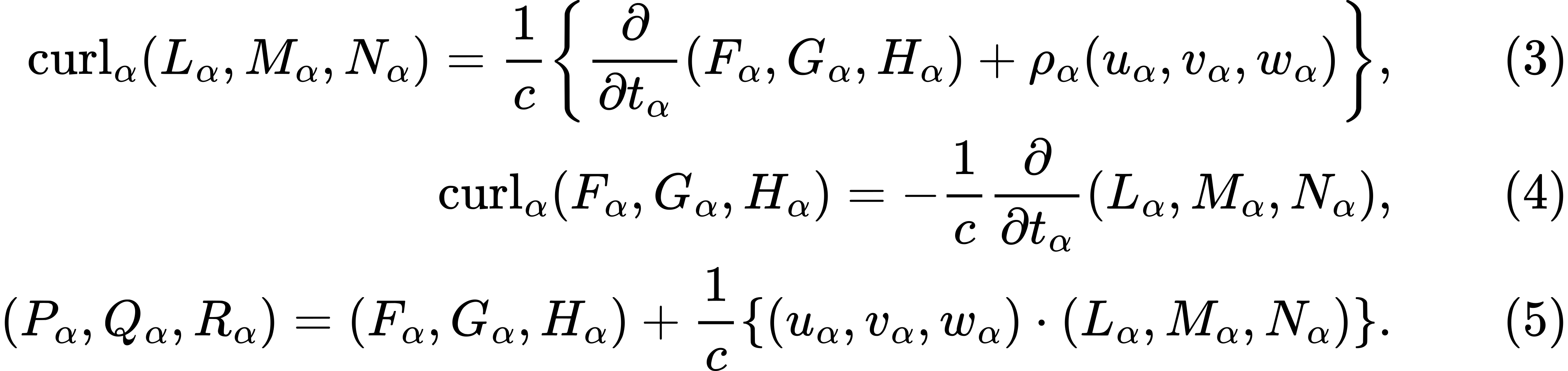
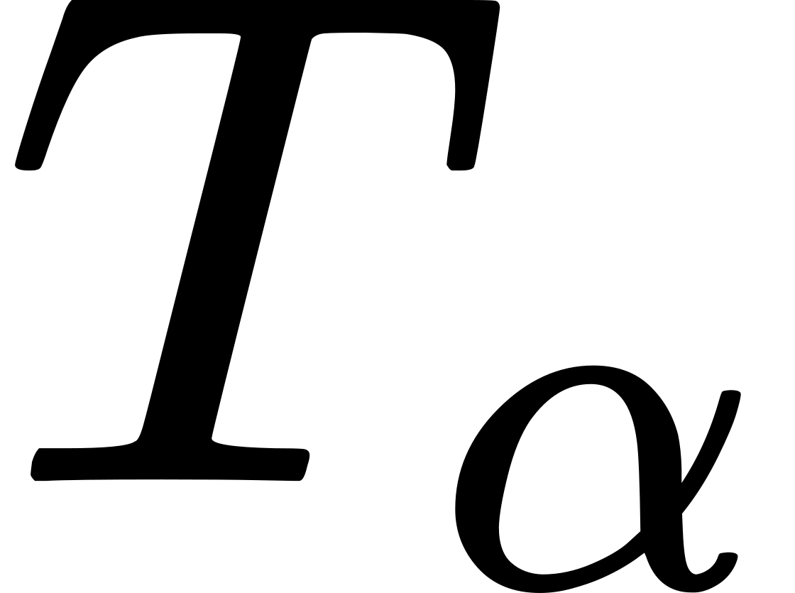 in the
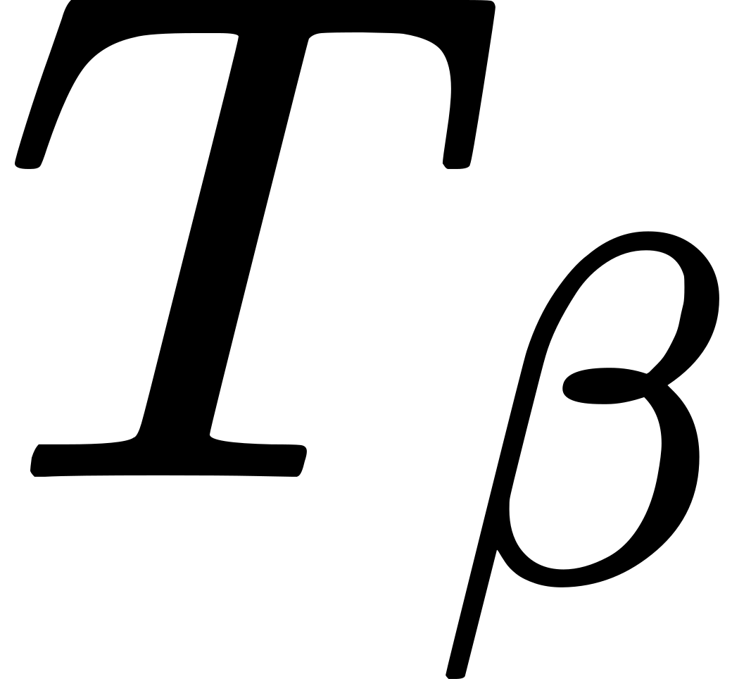 in the
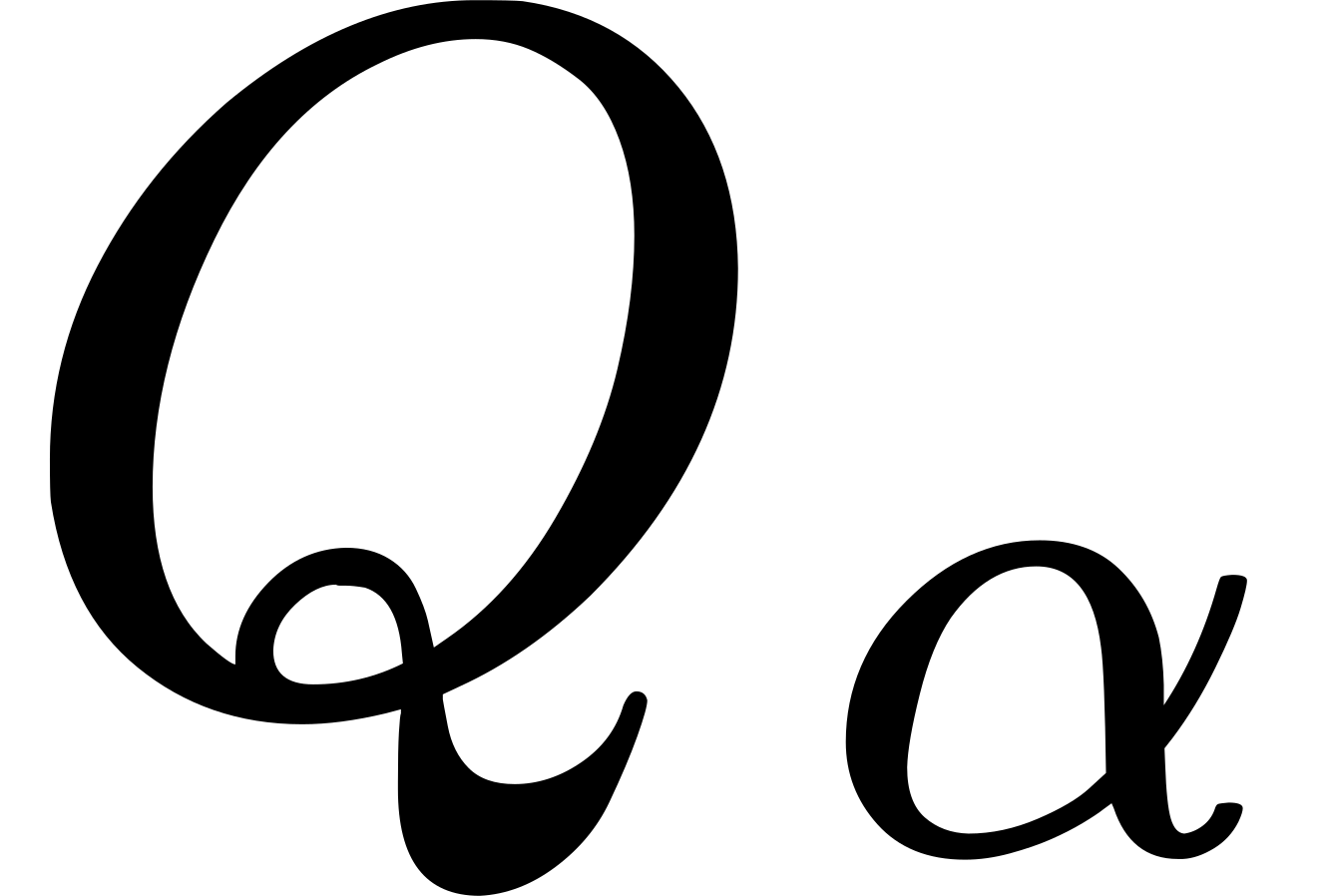 and
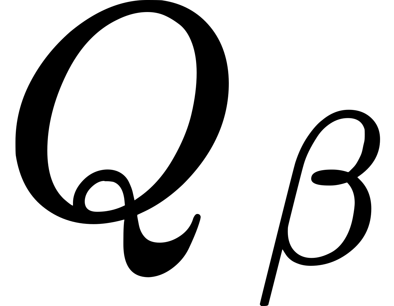 in the two spaces respectively.
Then according to the traditional scientific outlook,
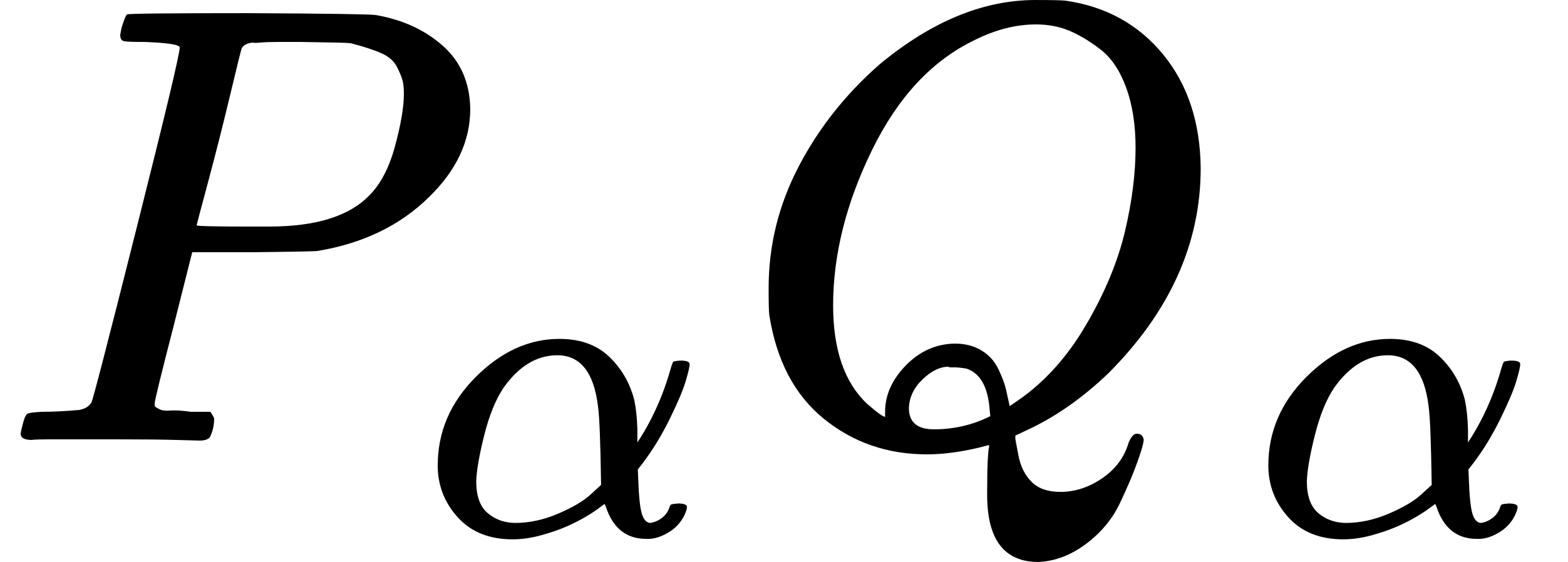 is (on this theory) equal to
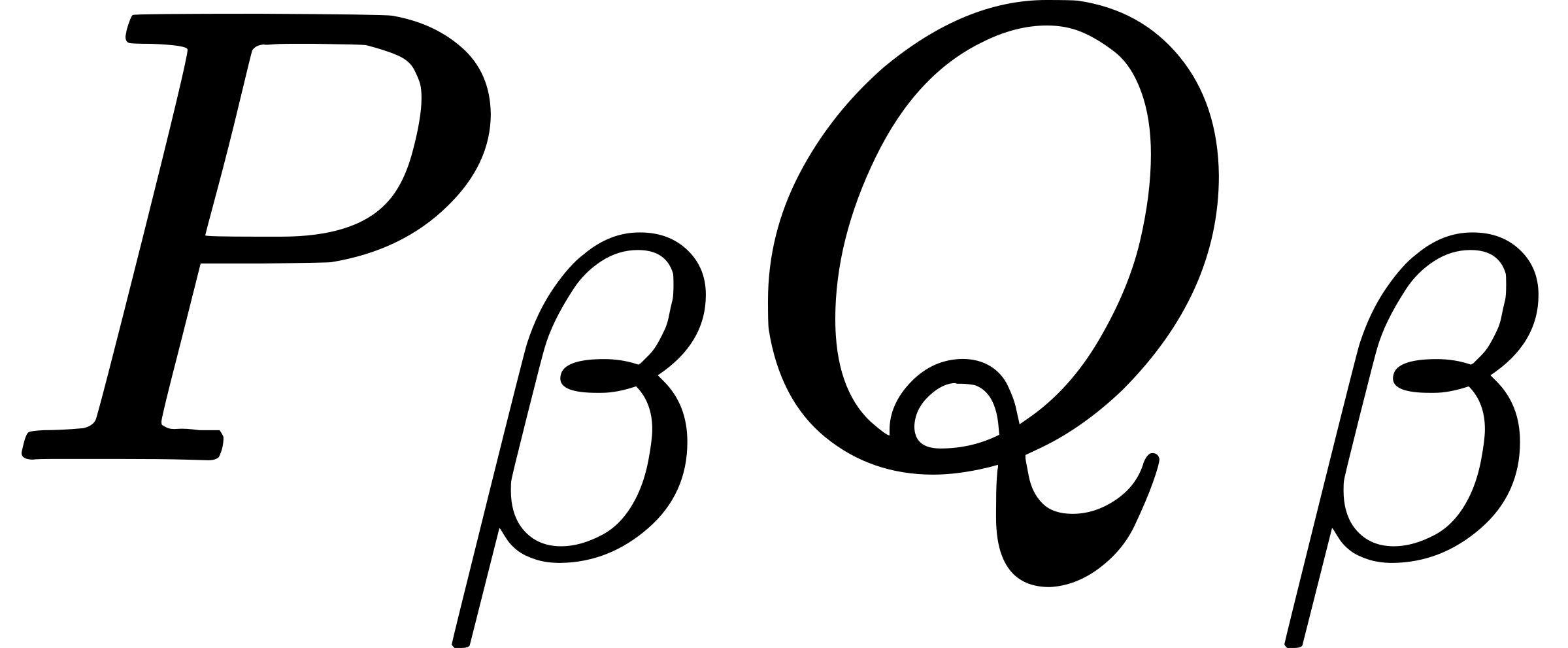 , because in fact they are symbols for the same
distance. But if the true distinction between the
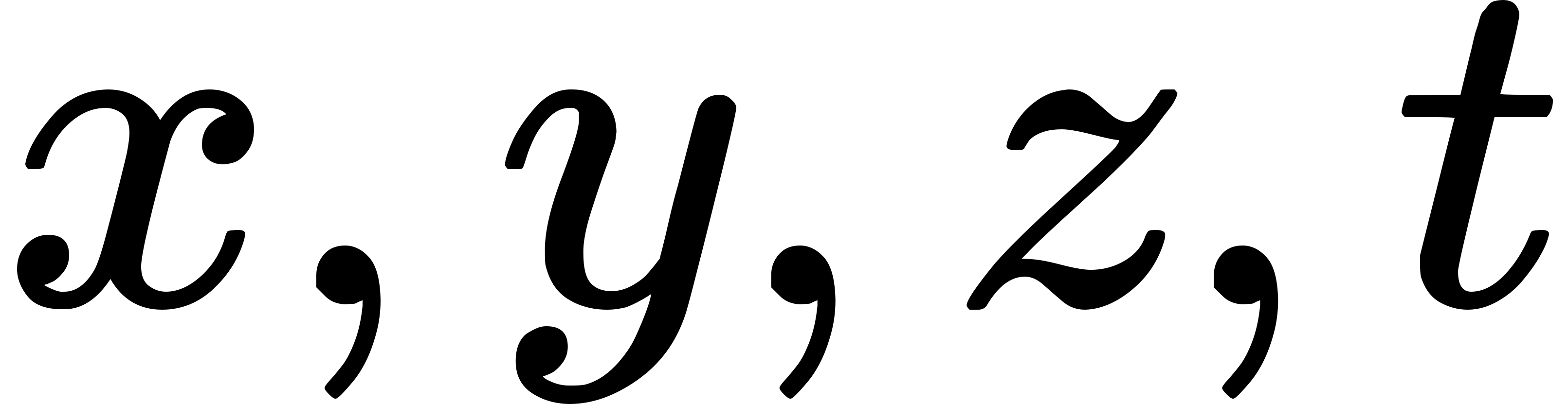 ) and interprets (
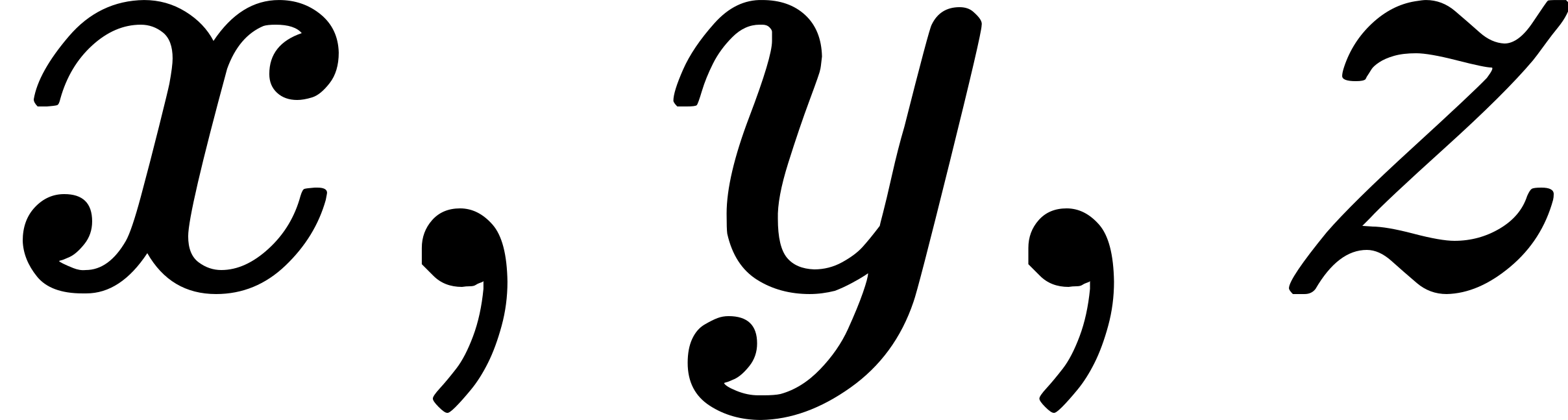 ) as space coordinates and
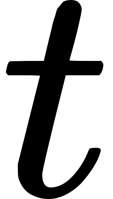 as a measure of time, merely on
the ground that some physical law is thereby expressed. This is not an
interpretation of what we mean by space and time. What we mean are
physical facts expressible in terms of immediate perceptions; and it is
incumbent on us to produce the perceptions of those facts as the
meanings of our terms.
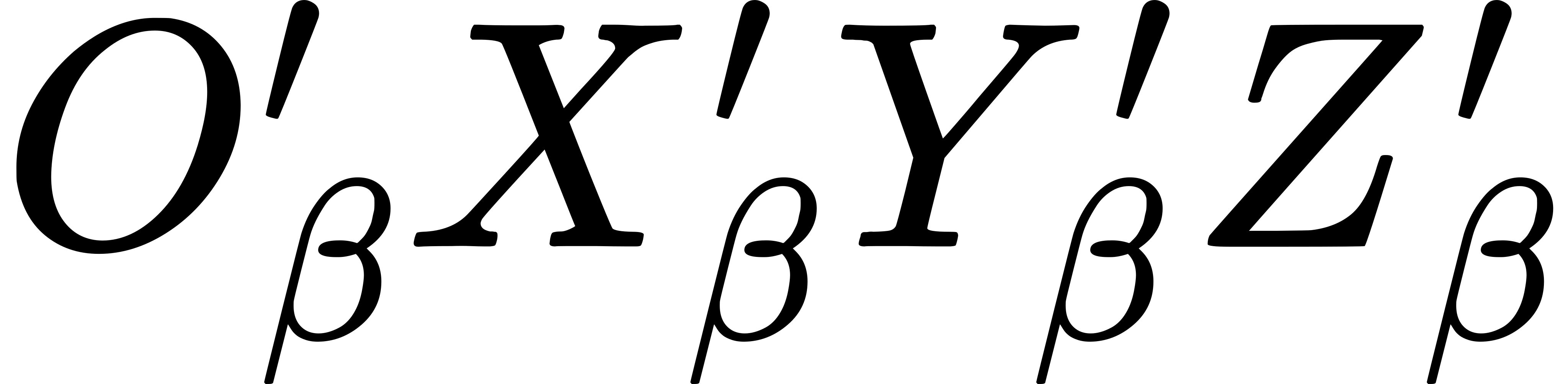 be the rectangular axis system in the space of
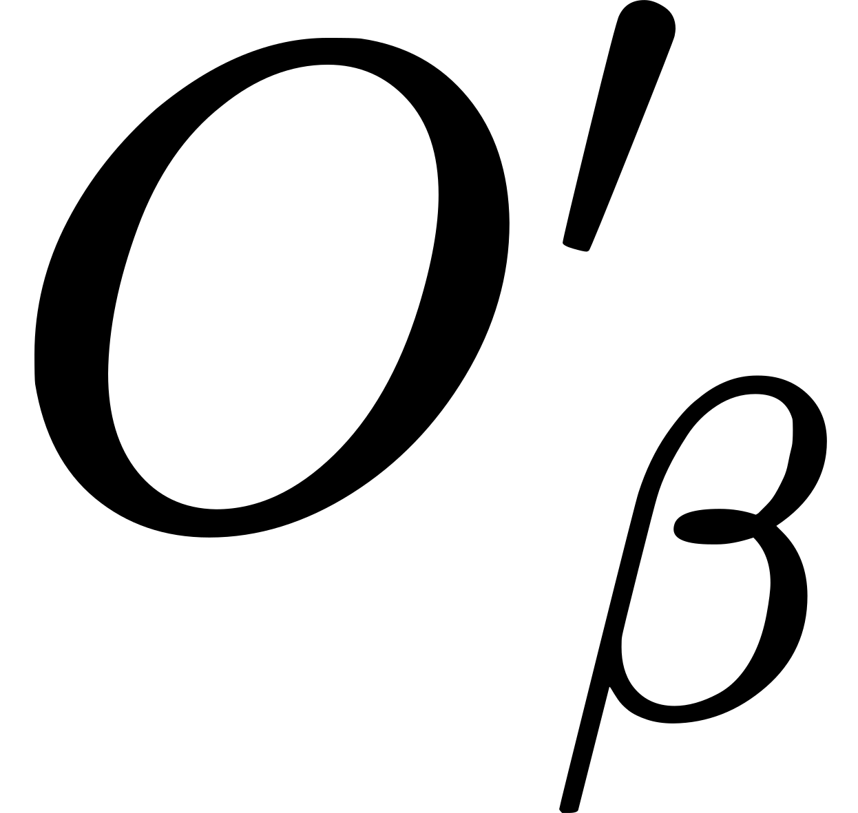
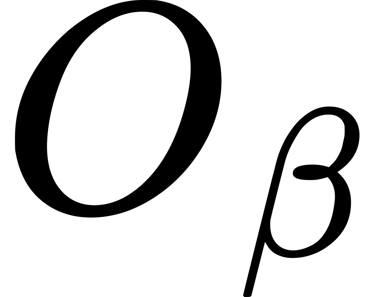 in
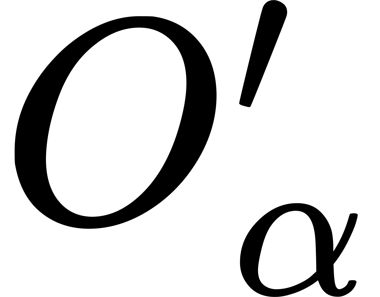
the space of
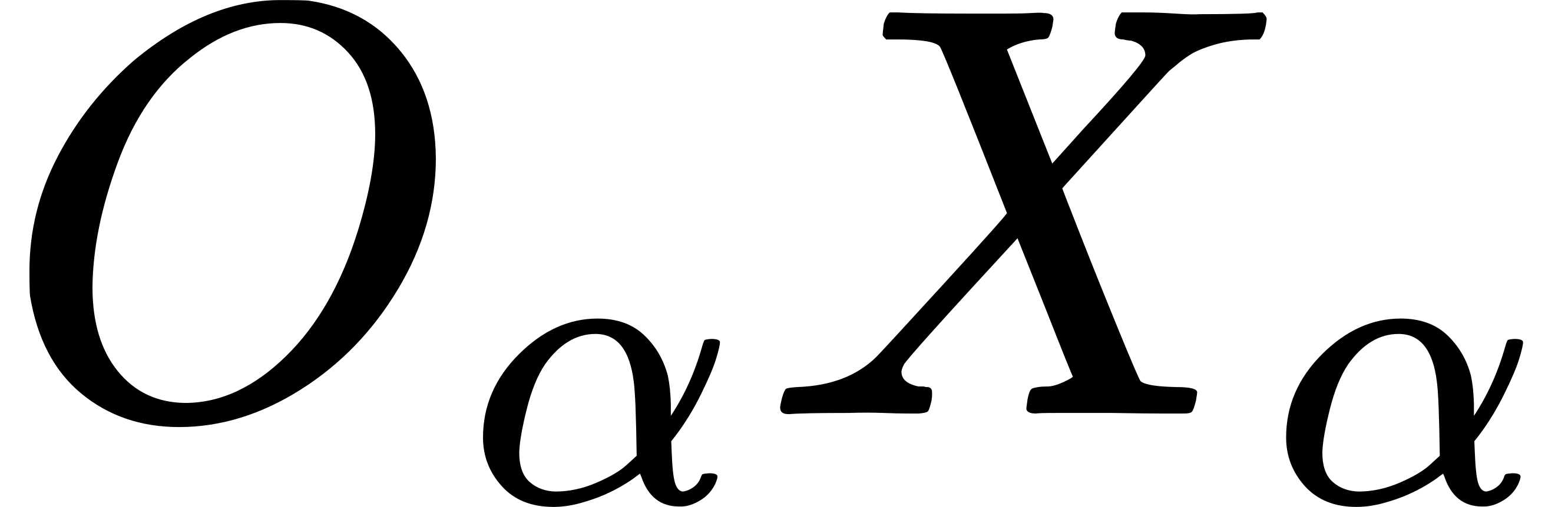
 in the space of
 in the space of
 be in the direction of the motion of
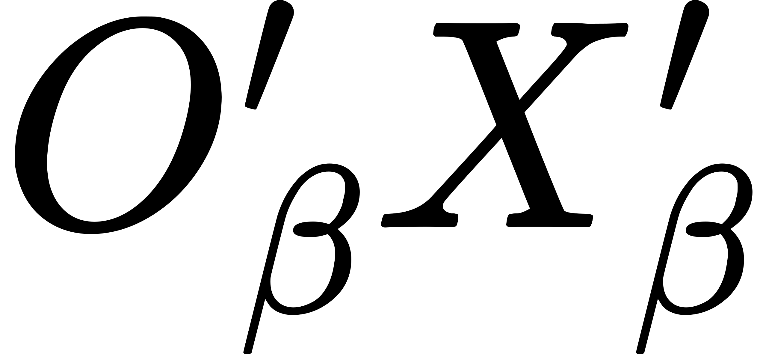 be in the direction reversed of
the motion of
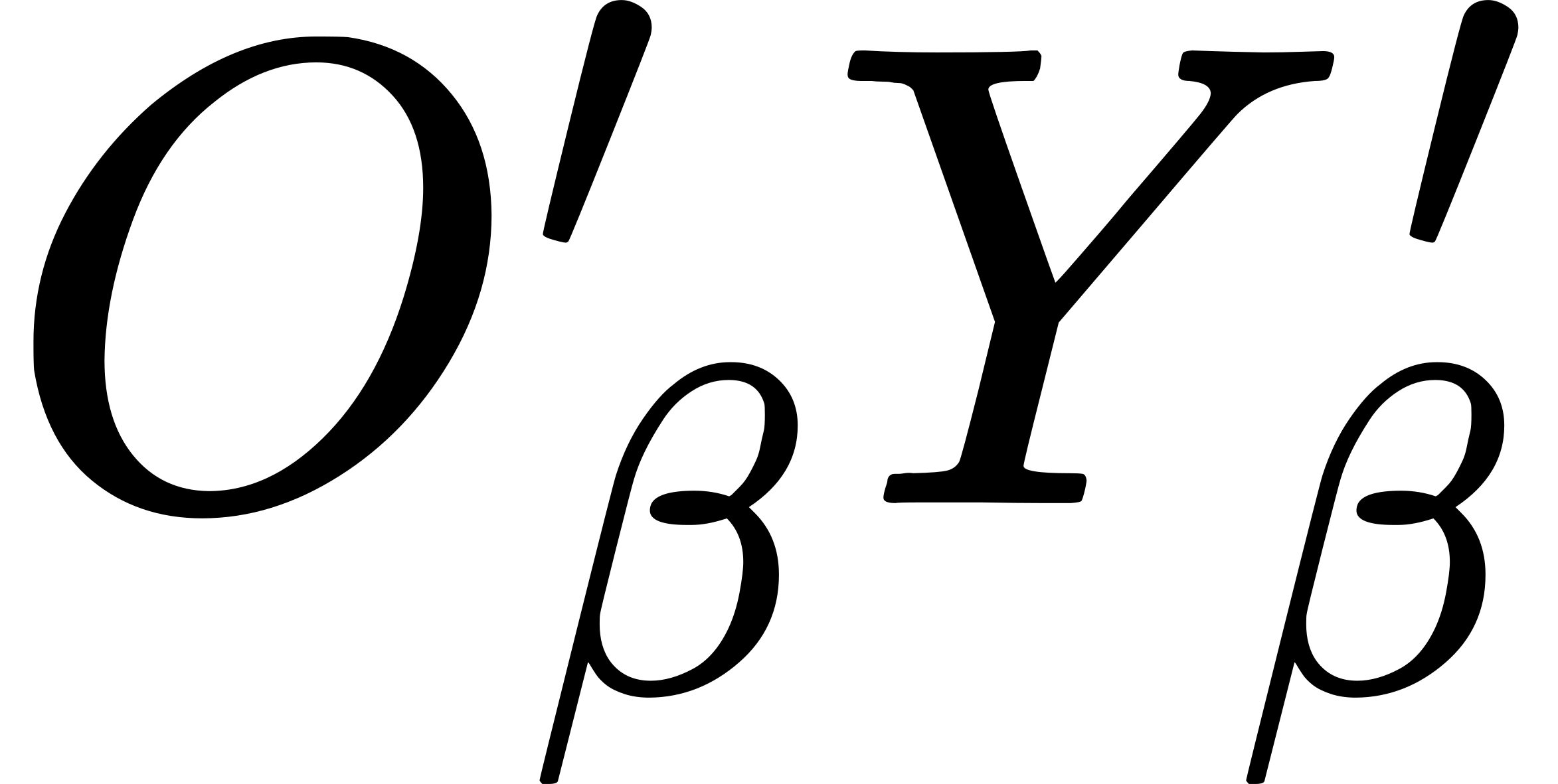 and
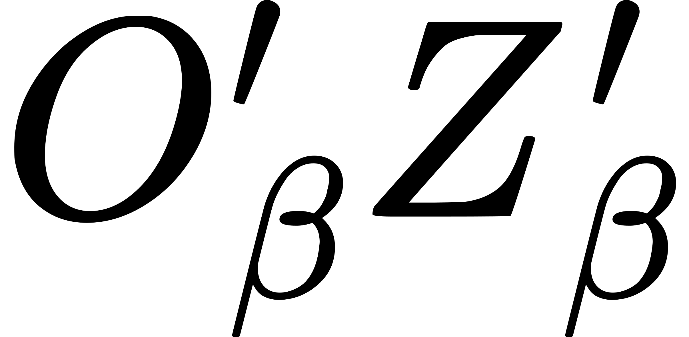 so that the event-particles
which happen at time
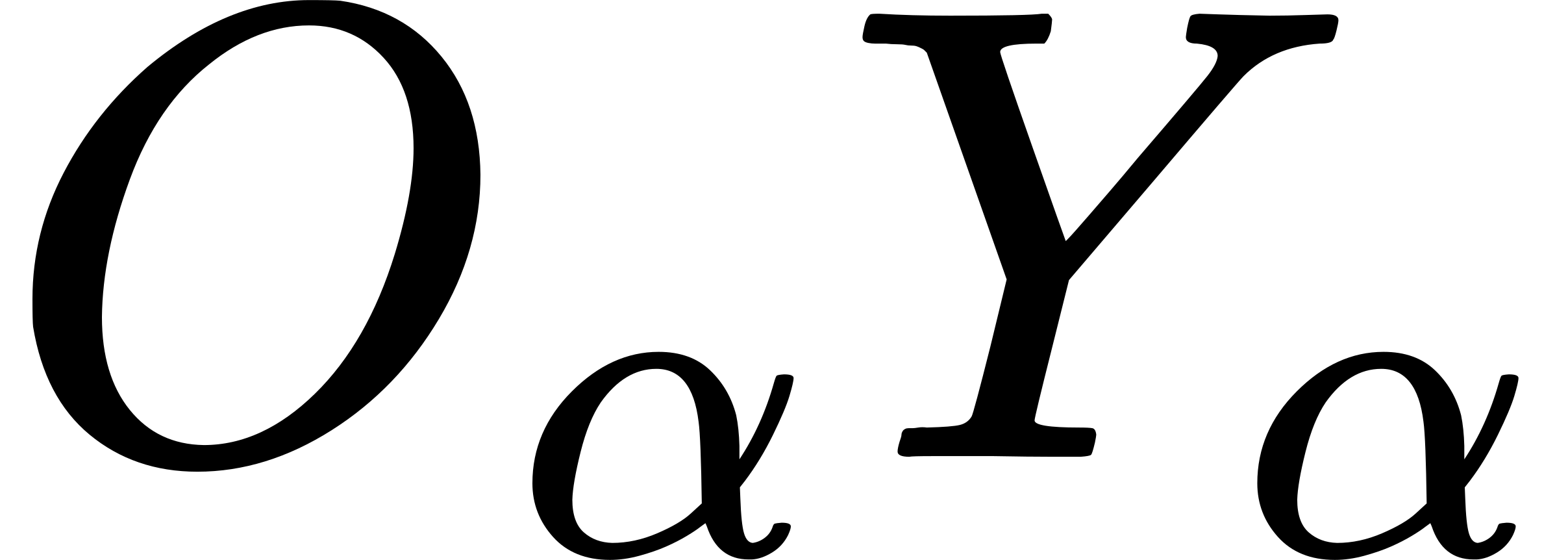 and
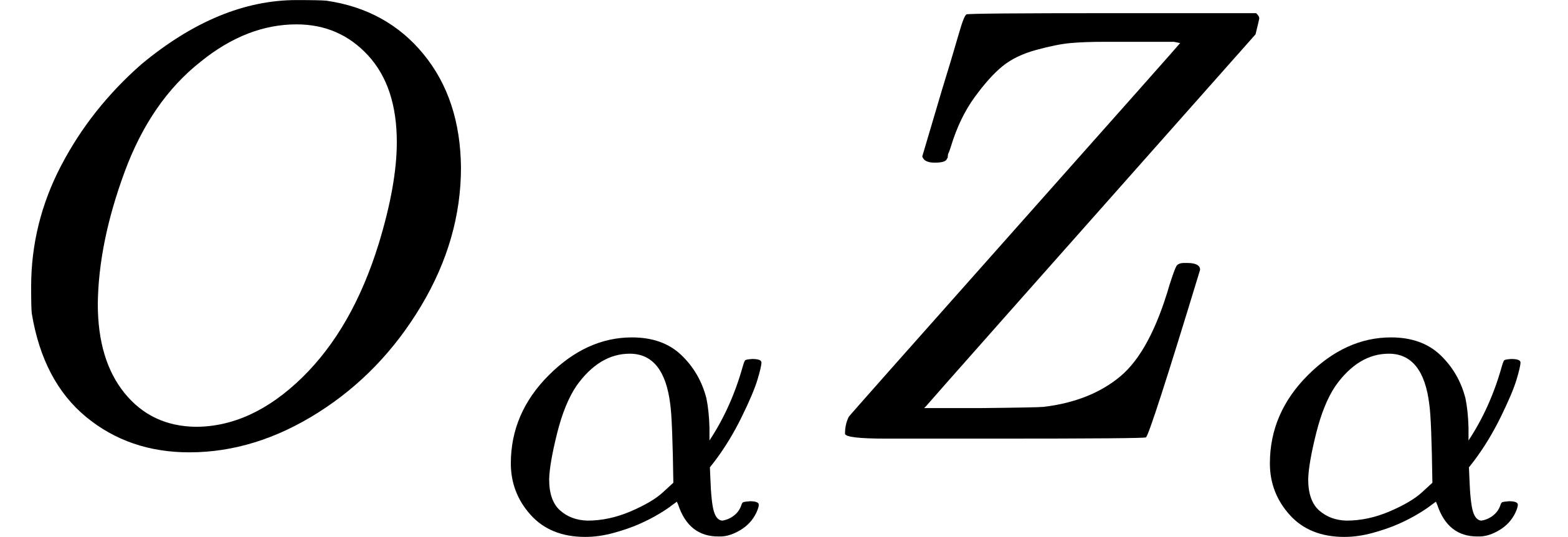 . Let
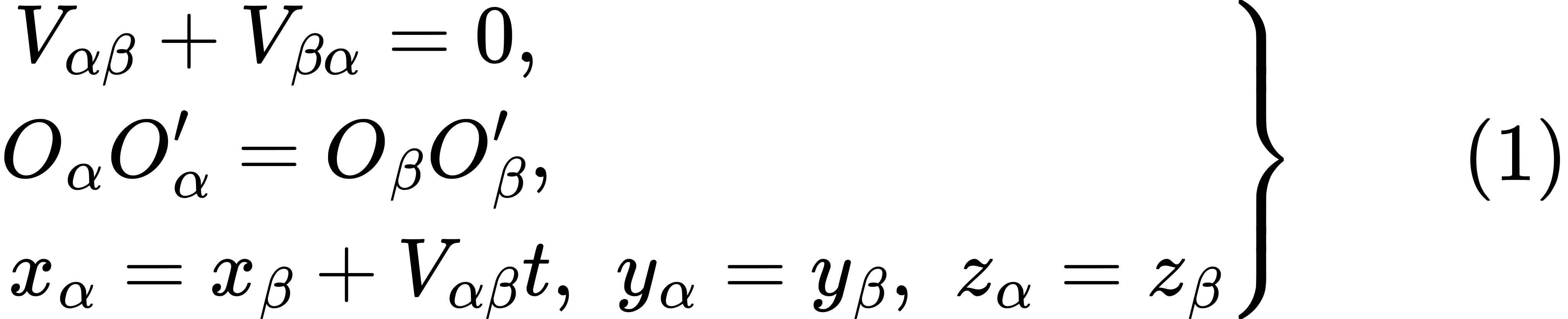
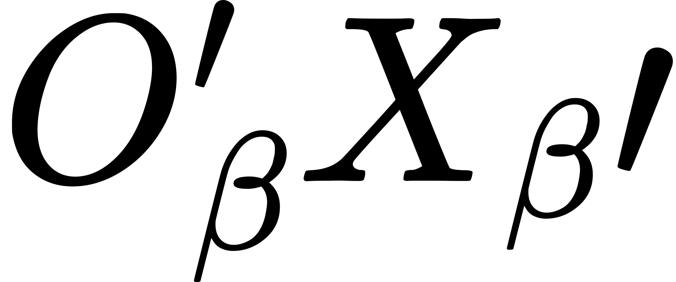 in the reverse direction of the
motion of
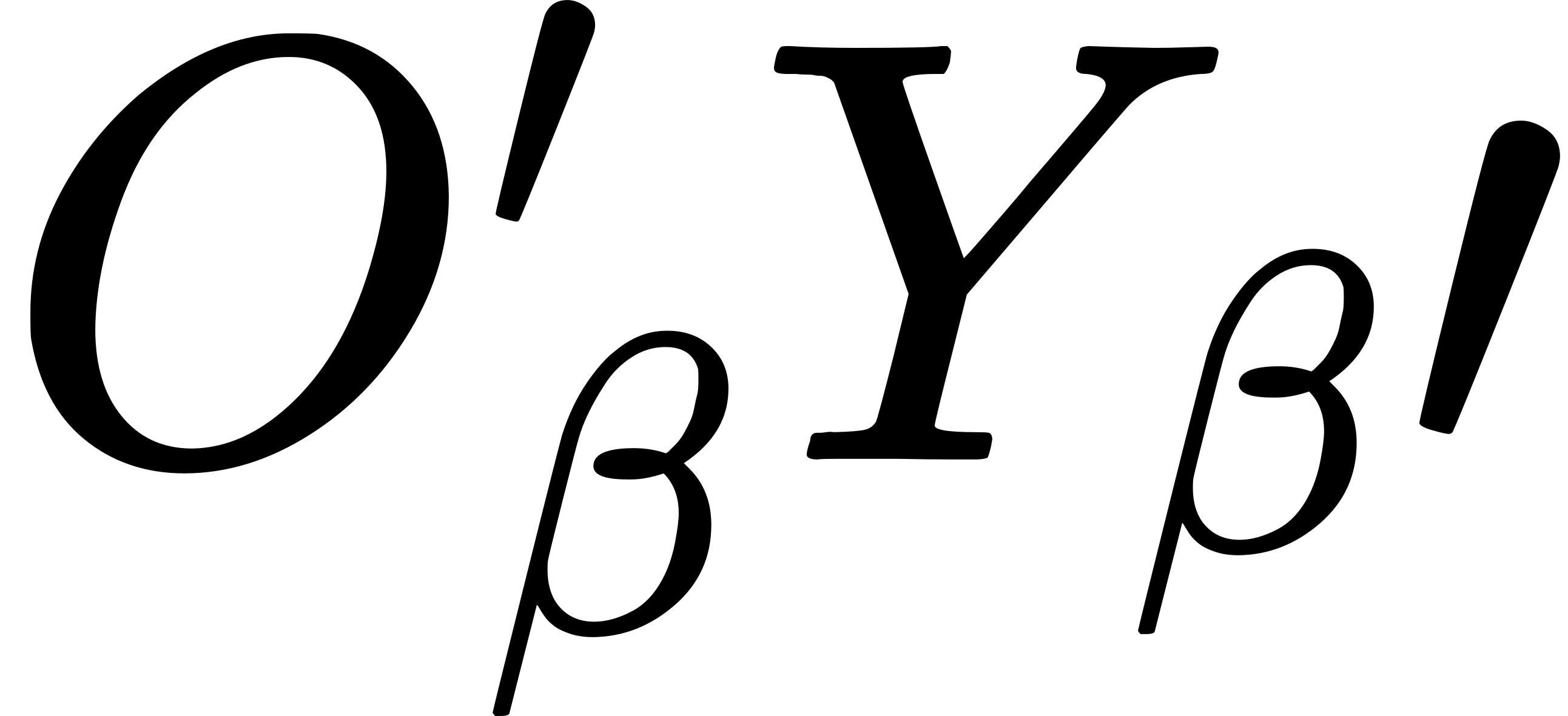 , and of
 , is defined and secured in
the same way as for Newtonian relativity.

 is small,

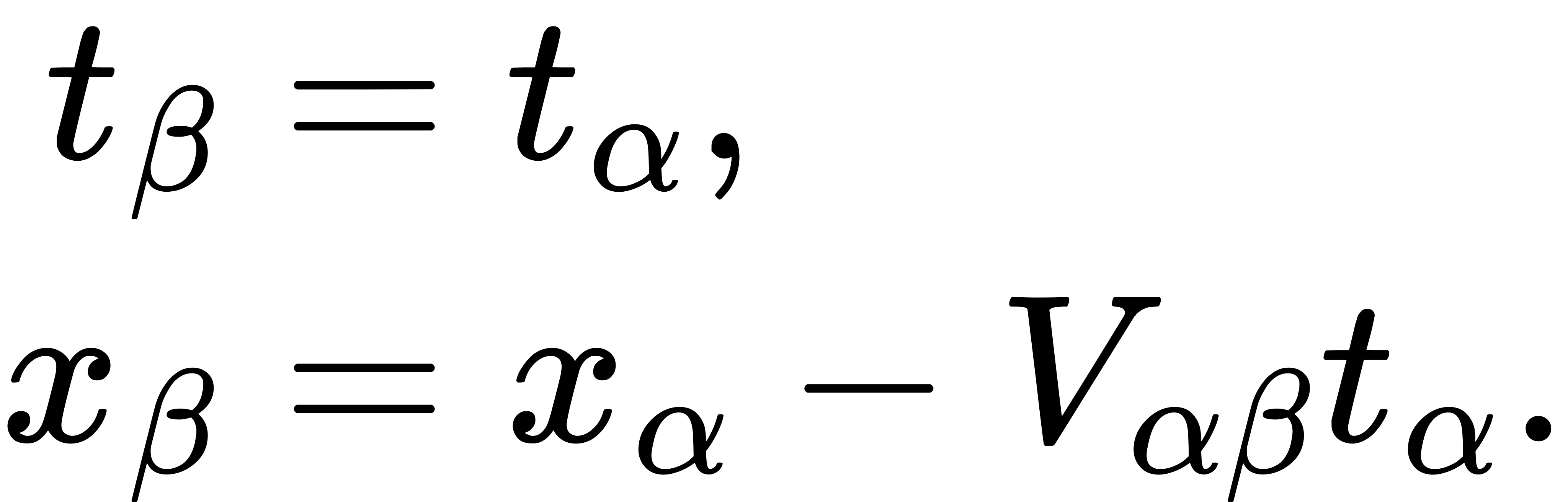
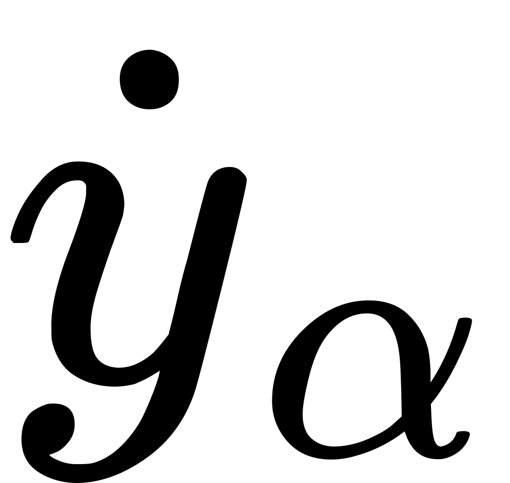 ,
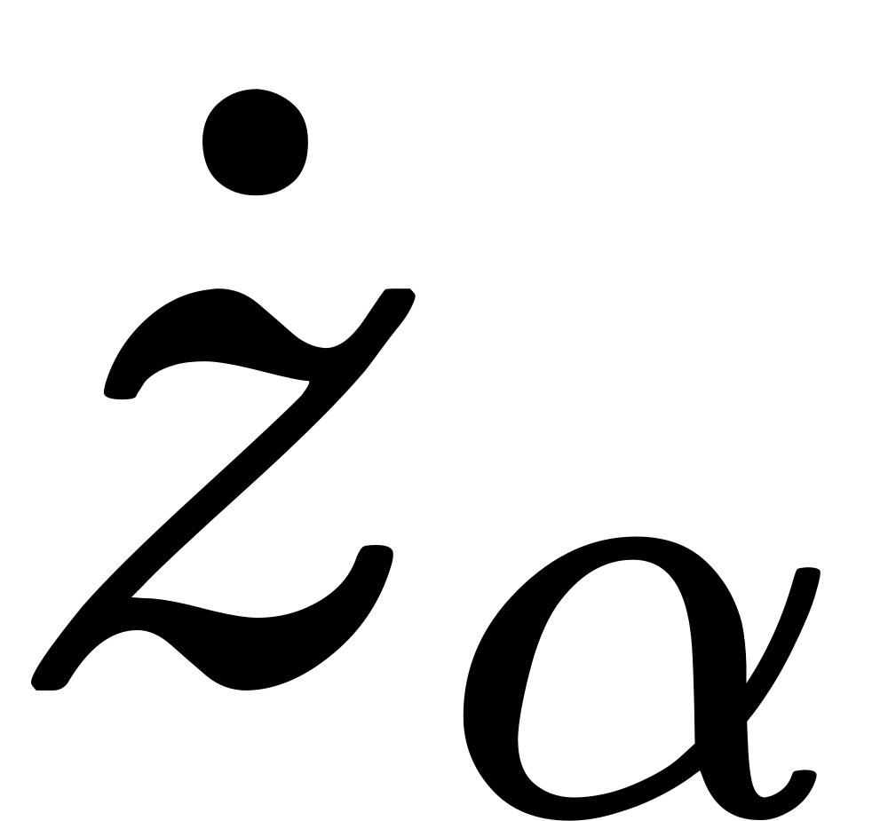 stand for
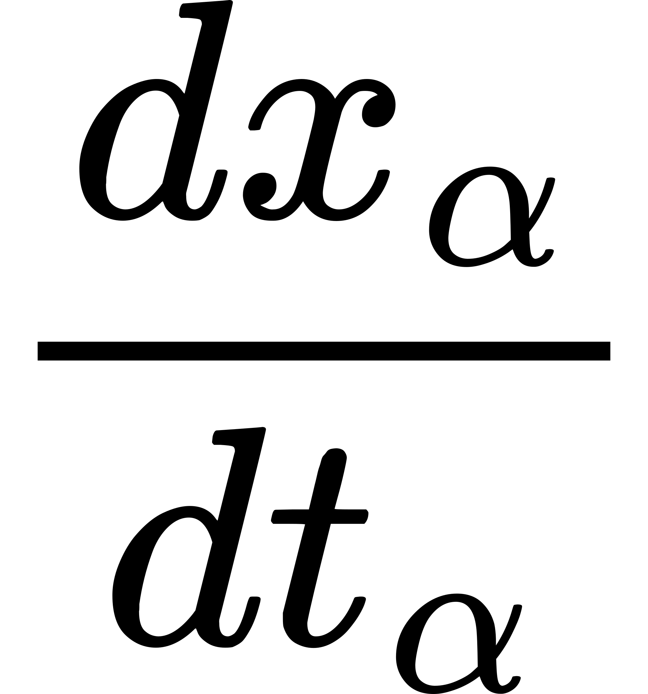 , etc., and
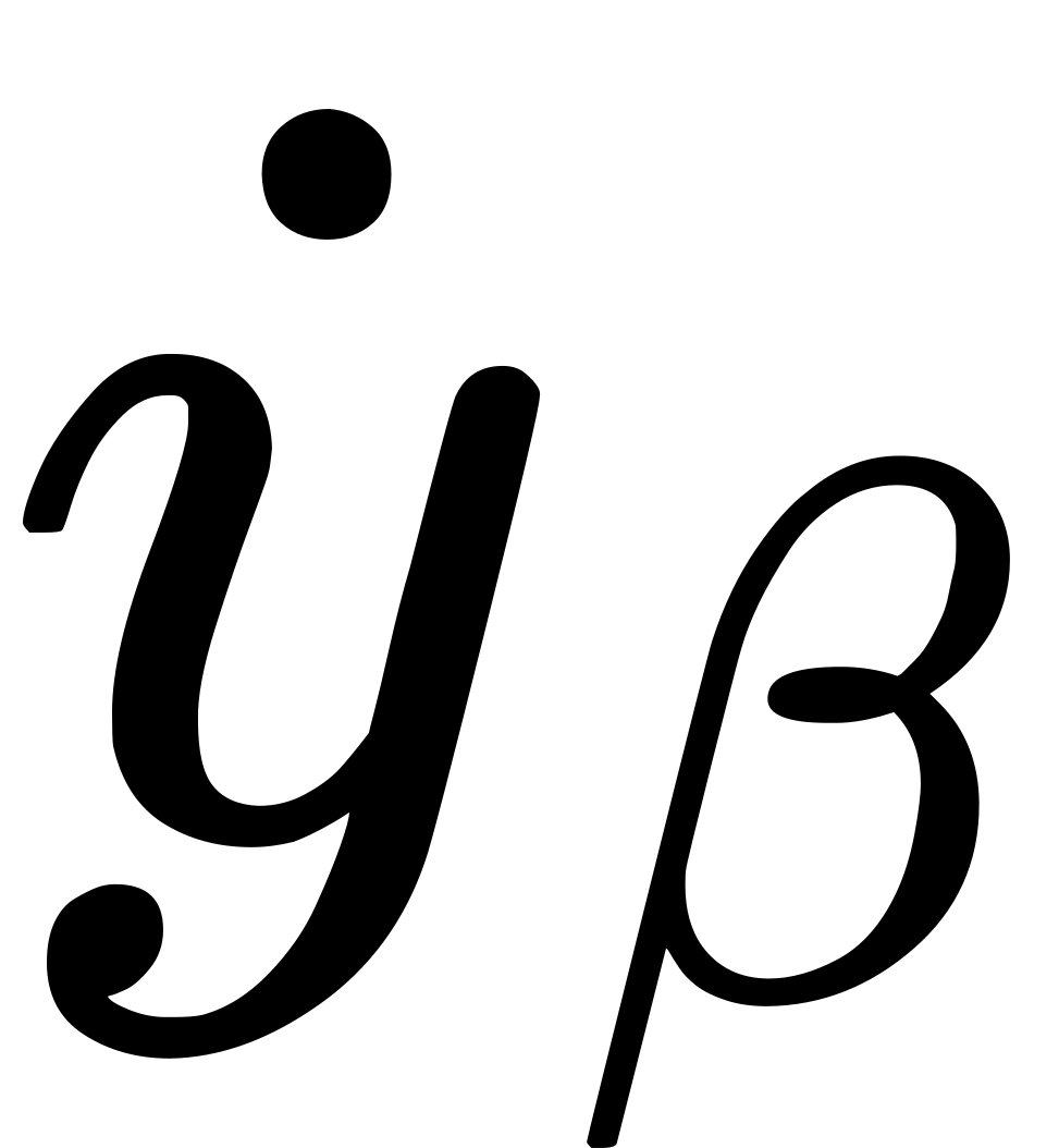 ,
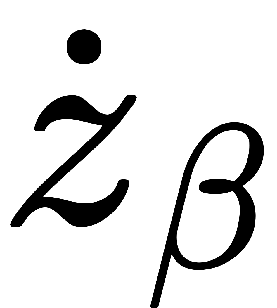 ,
for
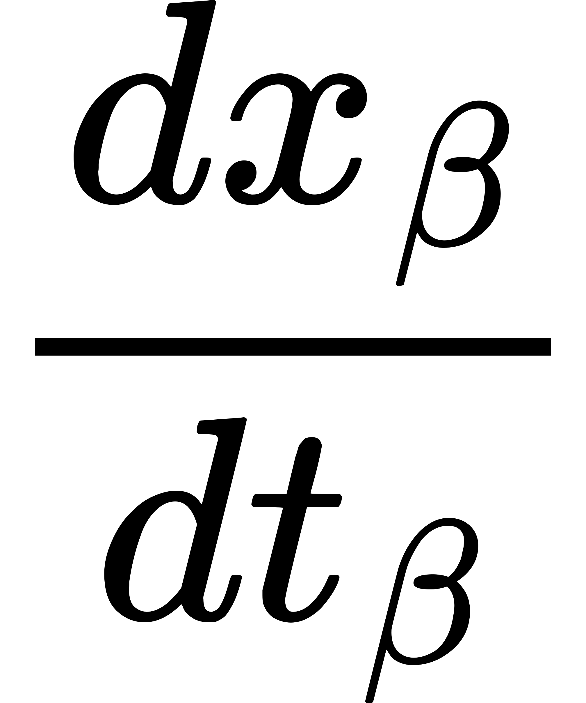 , etc.
Then it follows immediately from the preceding formulae that
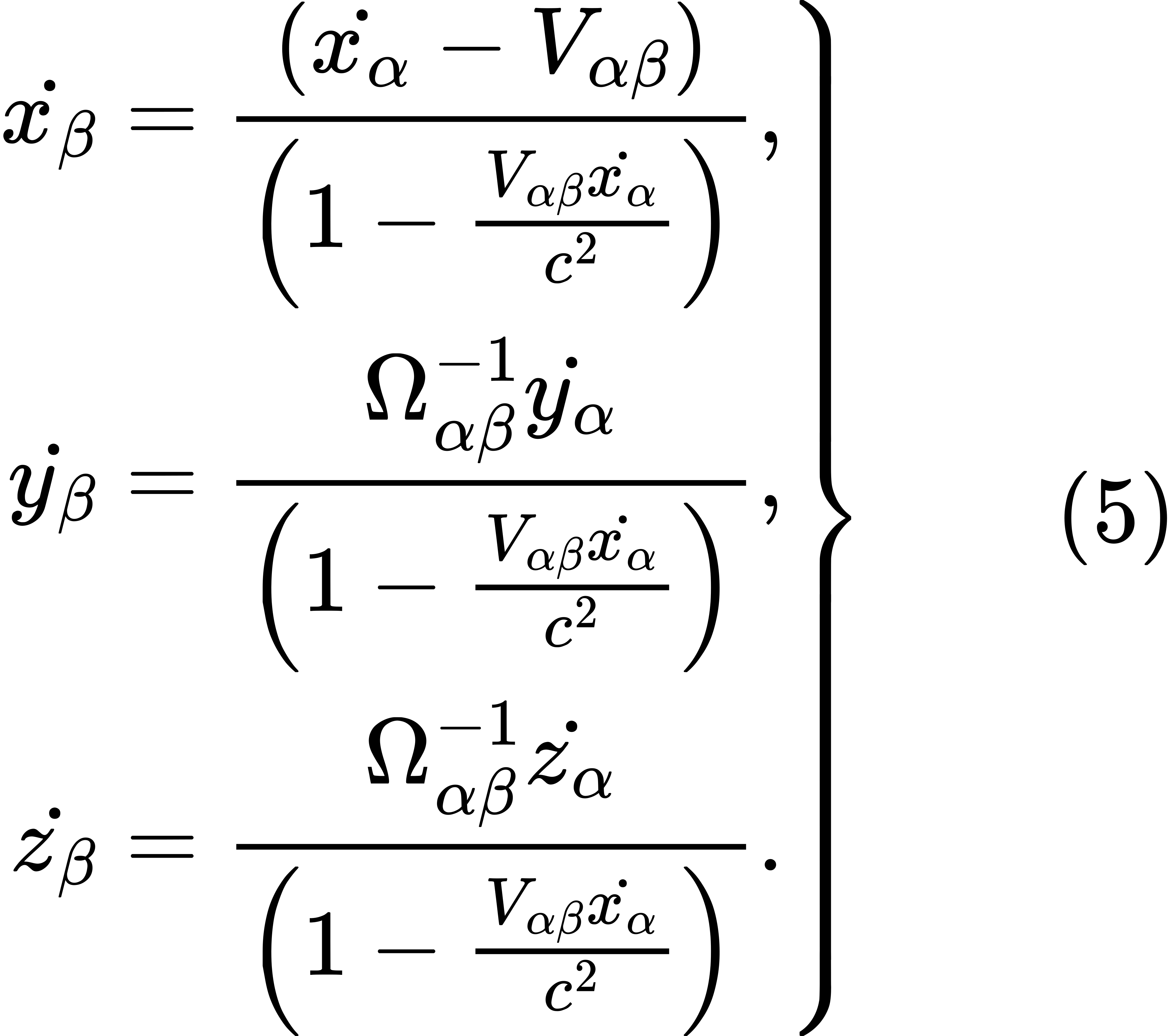
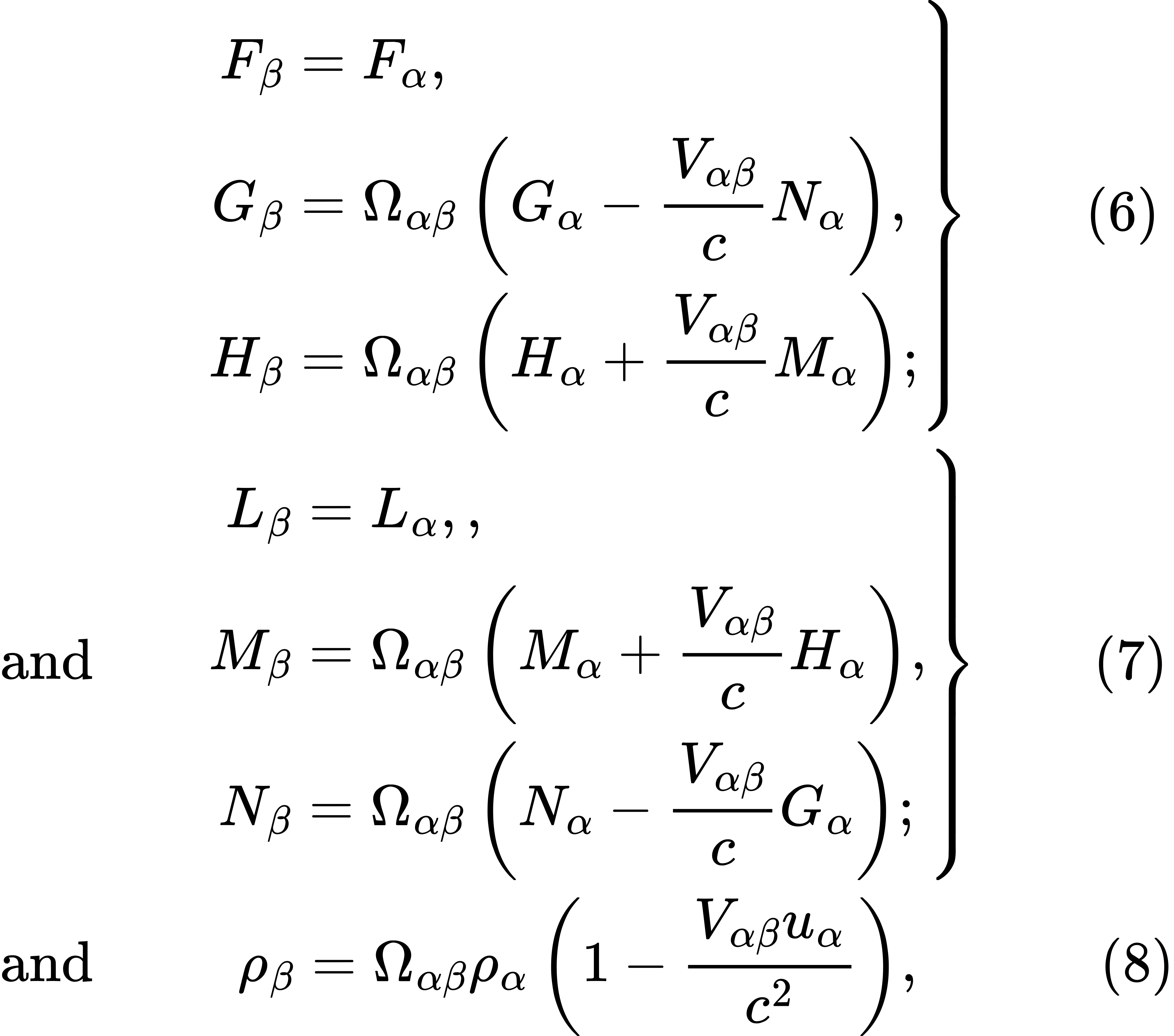


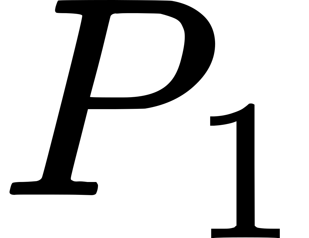 and
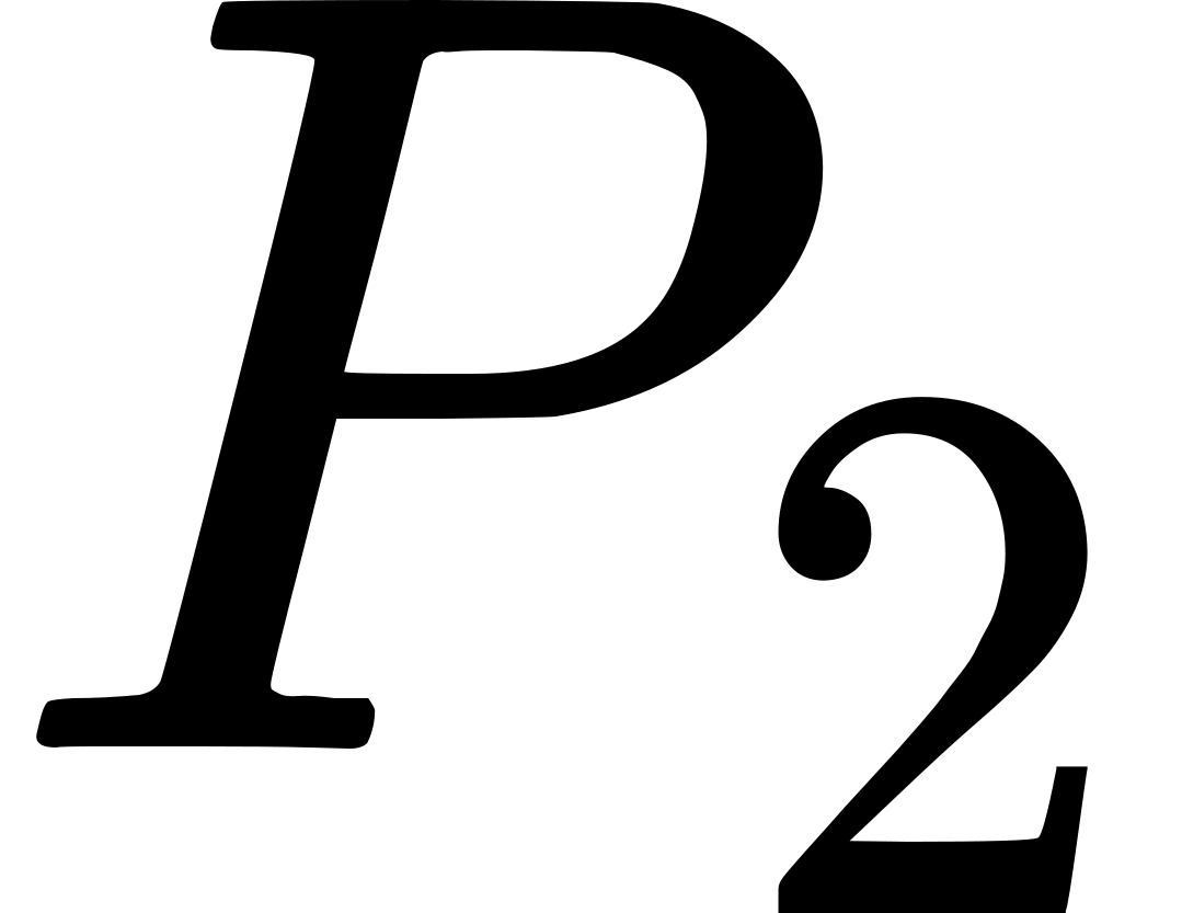 be two places,
the time-orders
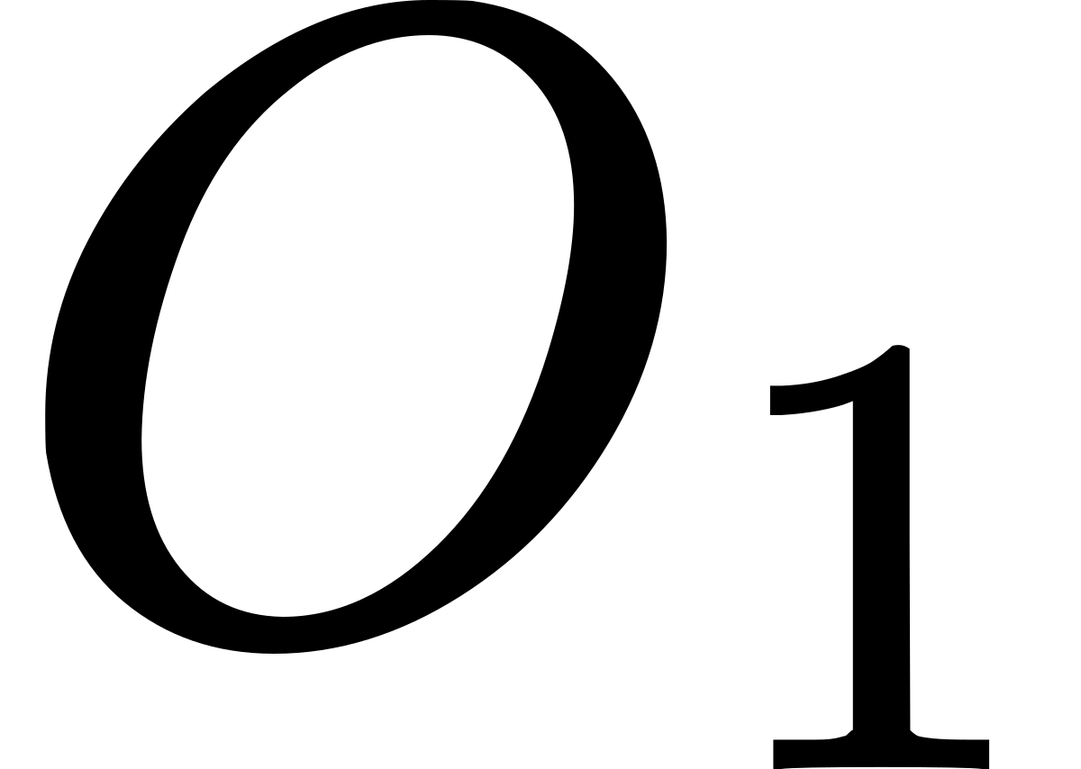 and
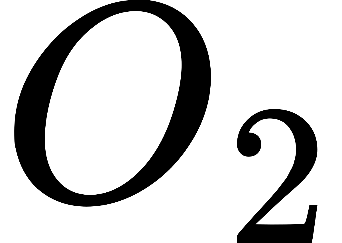 which belong to
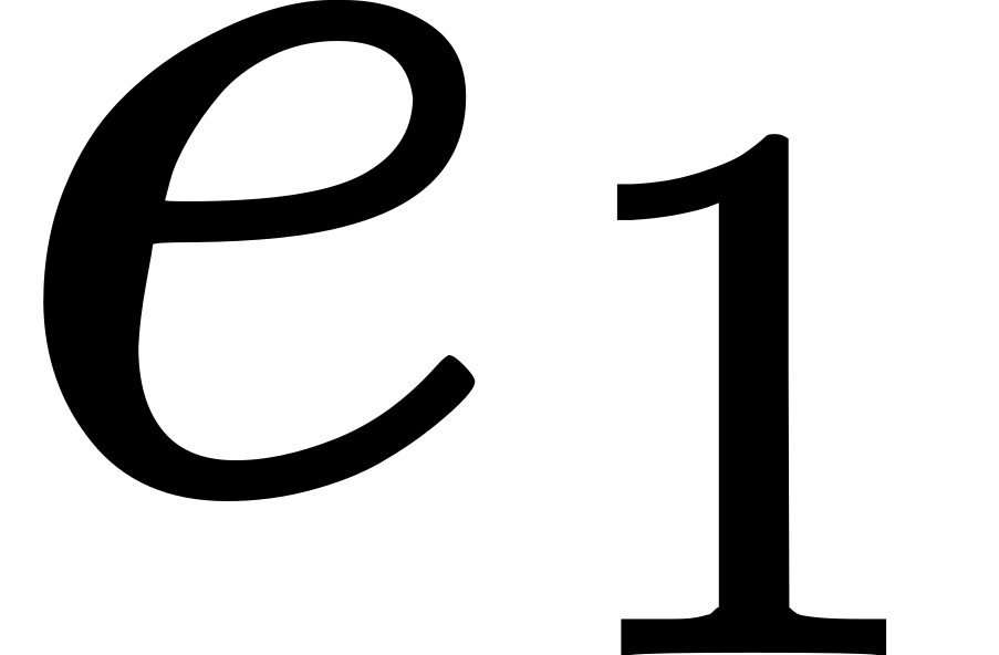 happens at
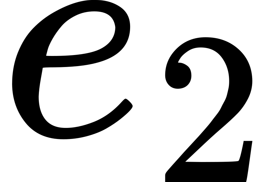 happens at
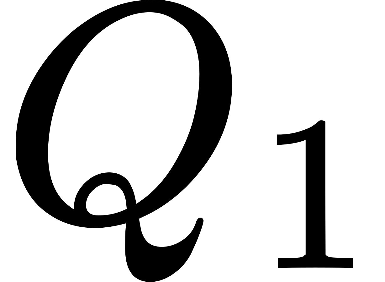 which
is rigidly connected with
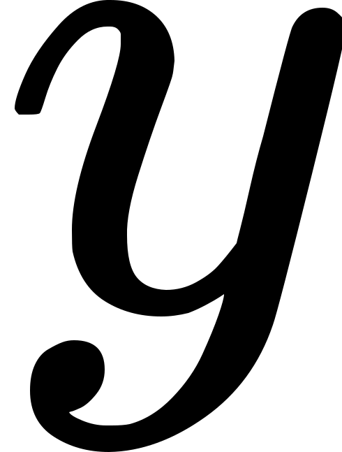 , i.e. in other
words
 be the given event, and
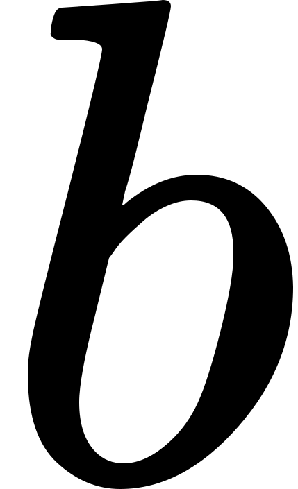 over
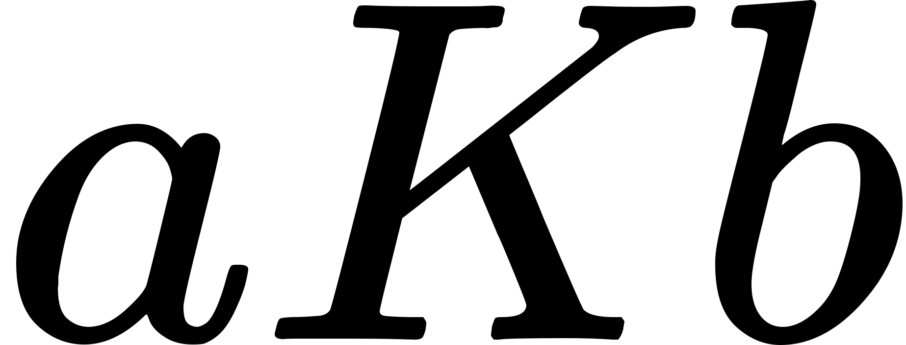 . Thus
'
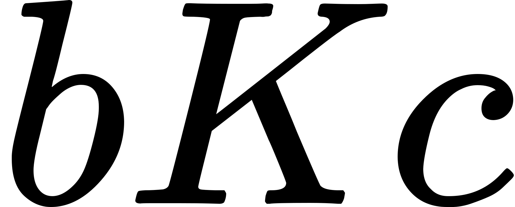 ,
then
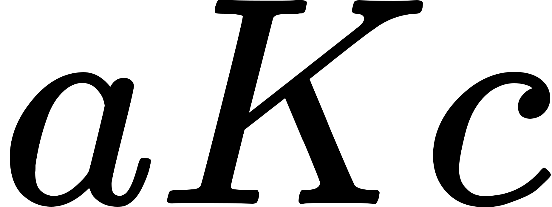 :
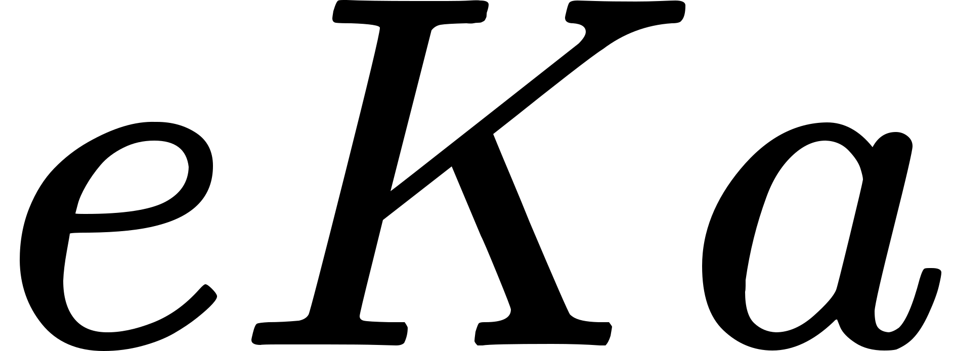 and
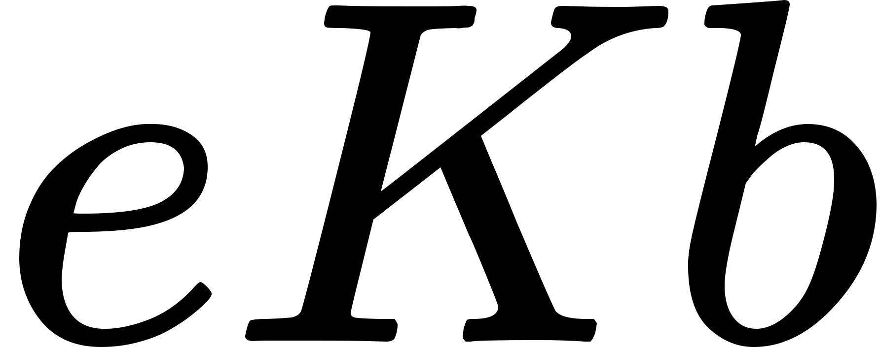 .
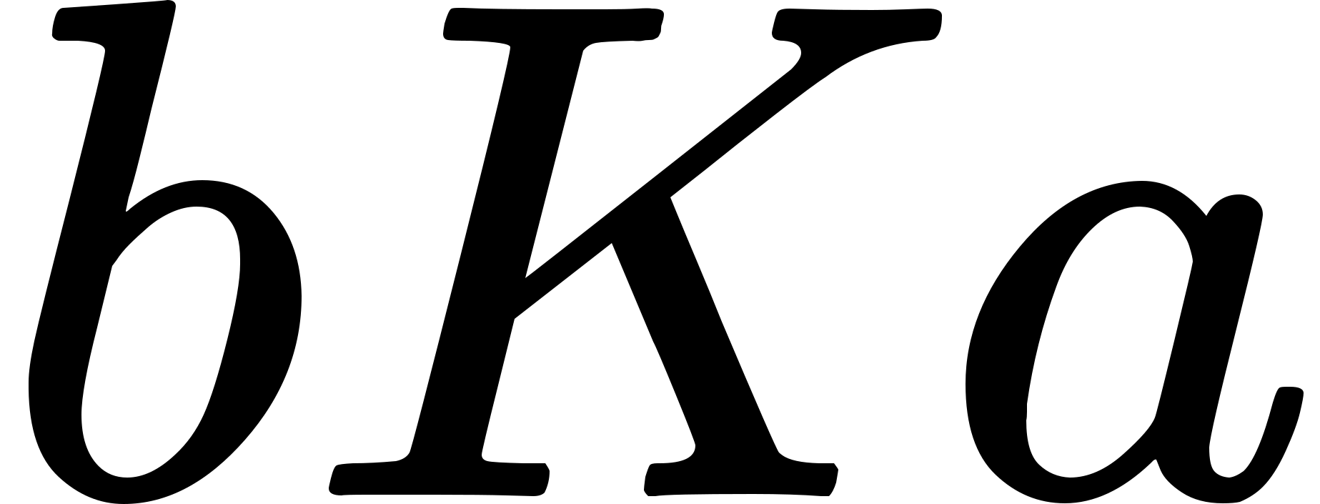 are inconsistent.
Properties (ii) and (v) and (vi) together postulate something like the
existence of an ether; but it is not necessary here to pursue the
analogy.
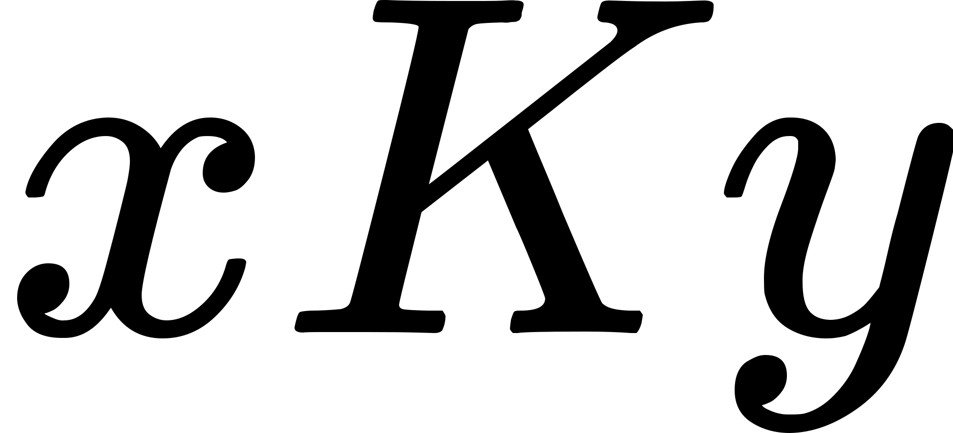 and


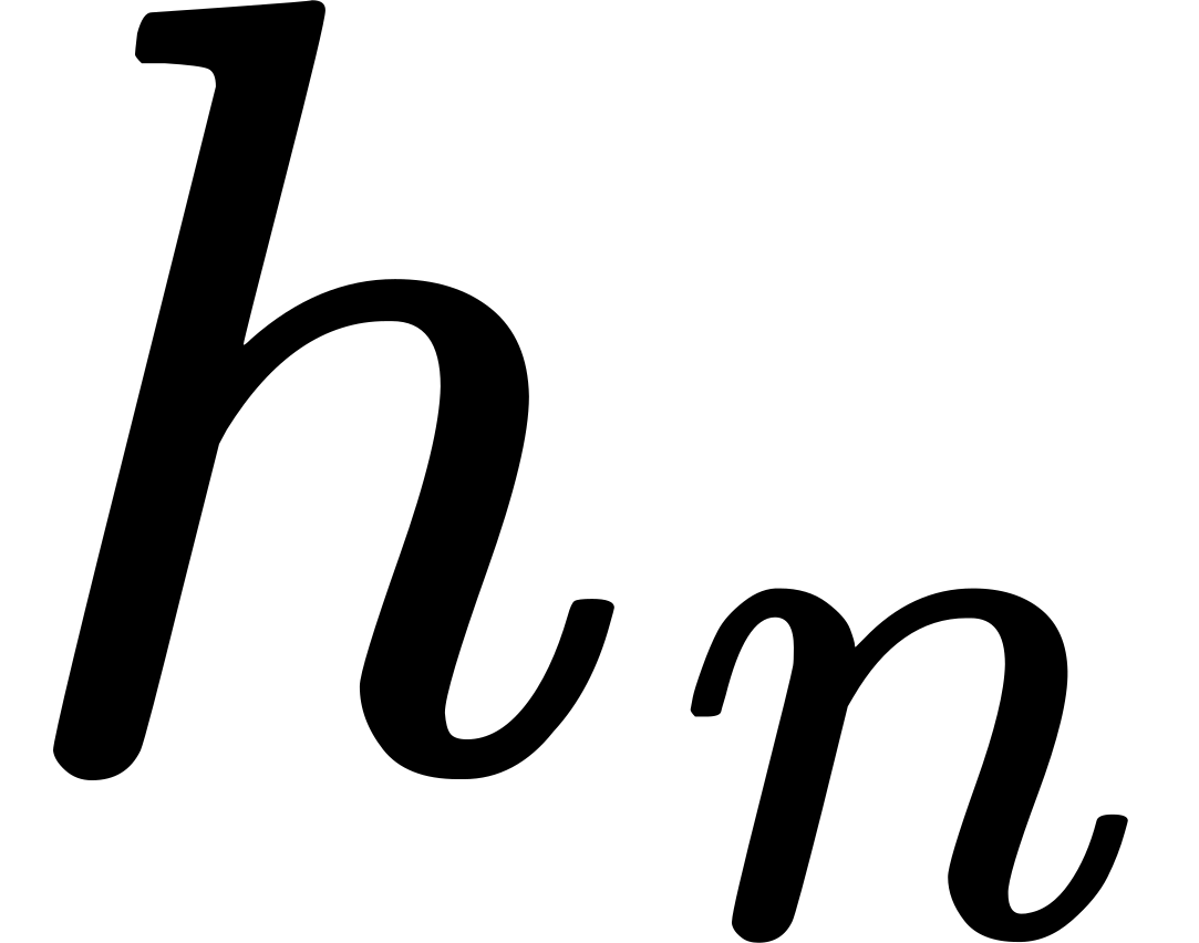 tend to zero as
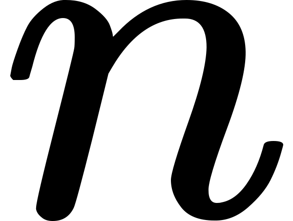 increases indefinitely. Then
the set forms an abstractive class.
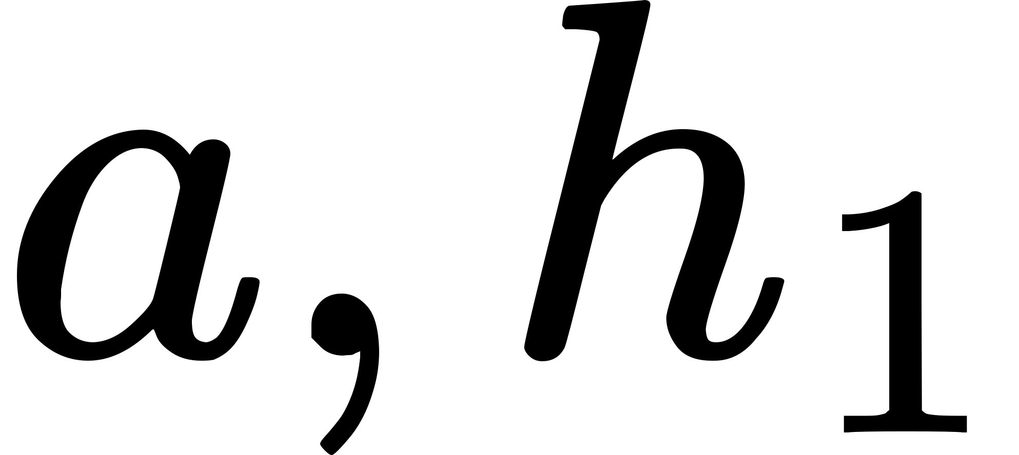 ), (
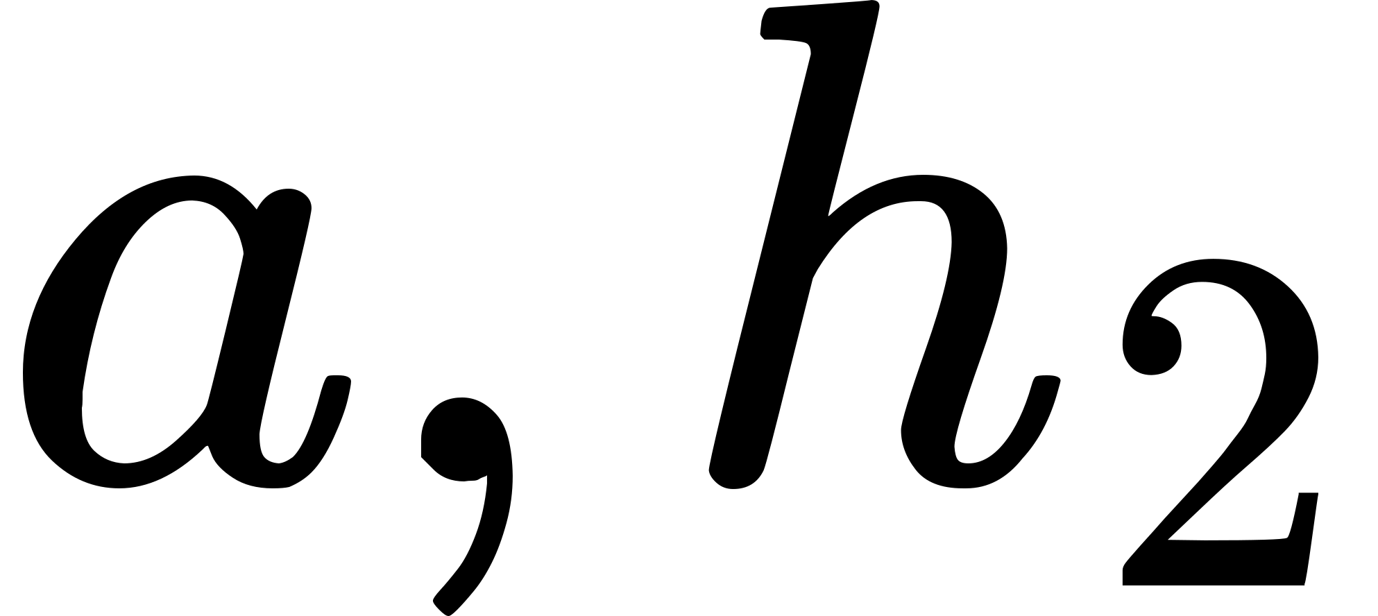 ),...(
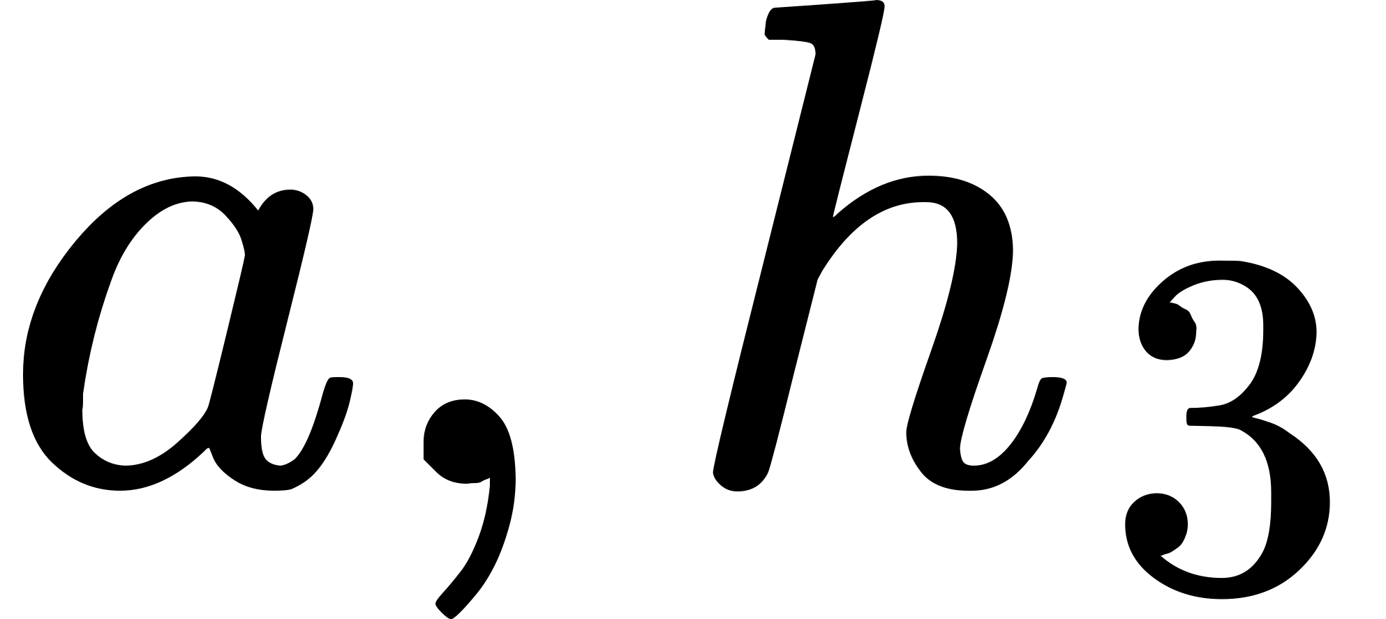 ),....
 ' [whatever condition '
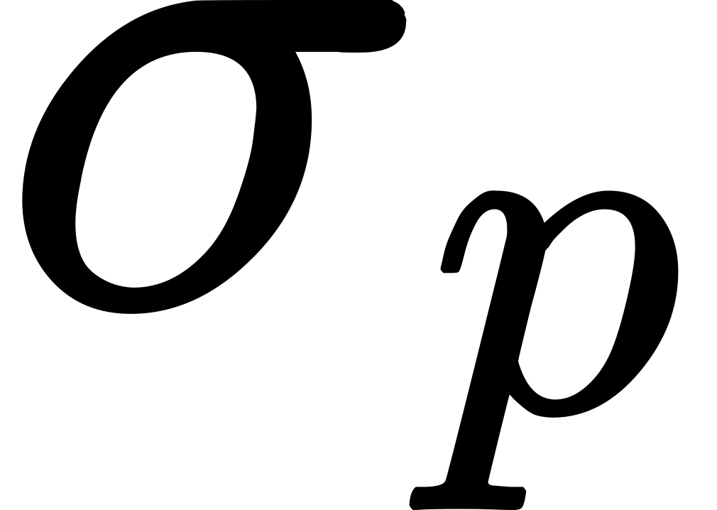 be the condition of 'being a
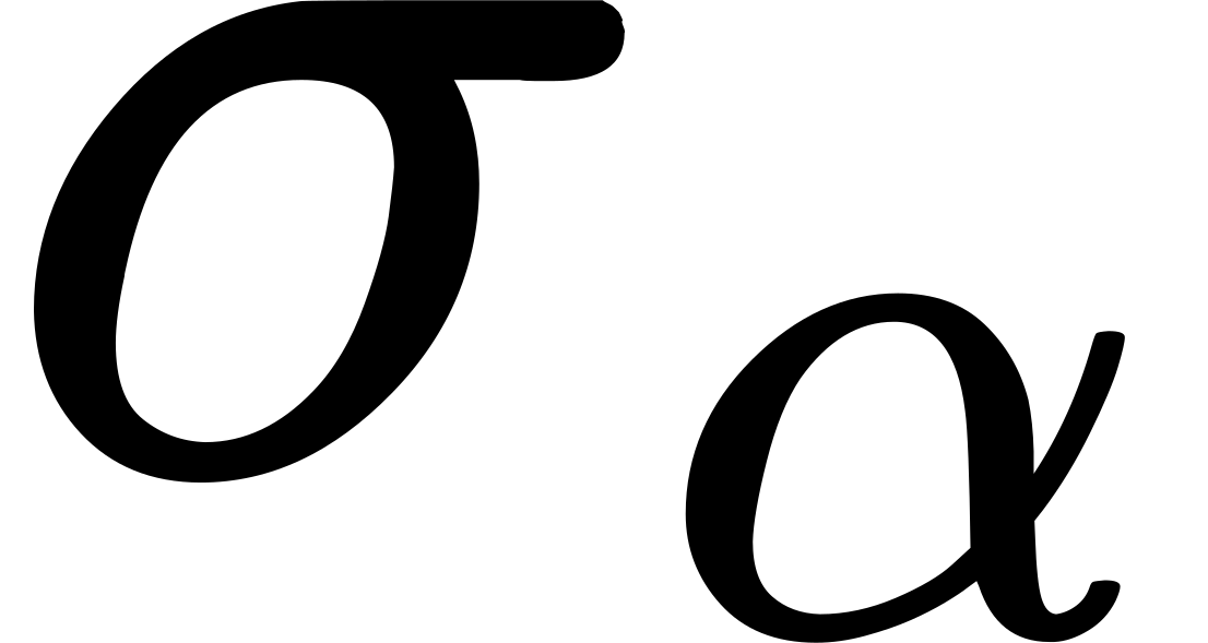 be the condition of 'being a
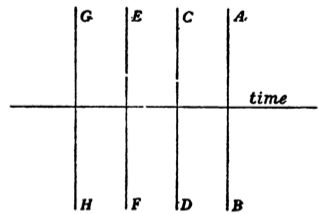
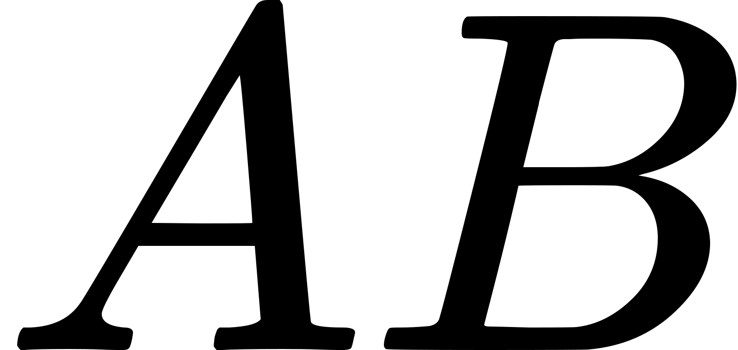 and
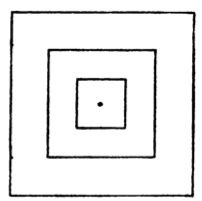
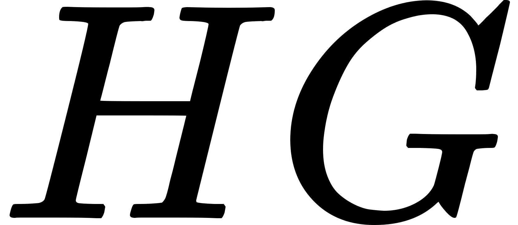 represents a duration. Also the area between
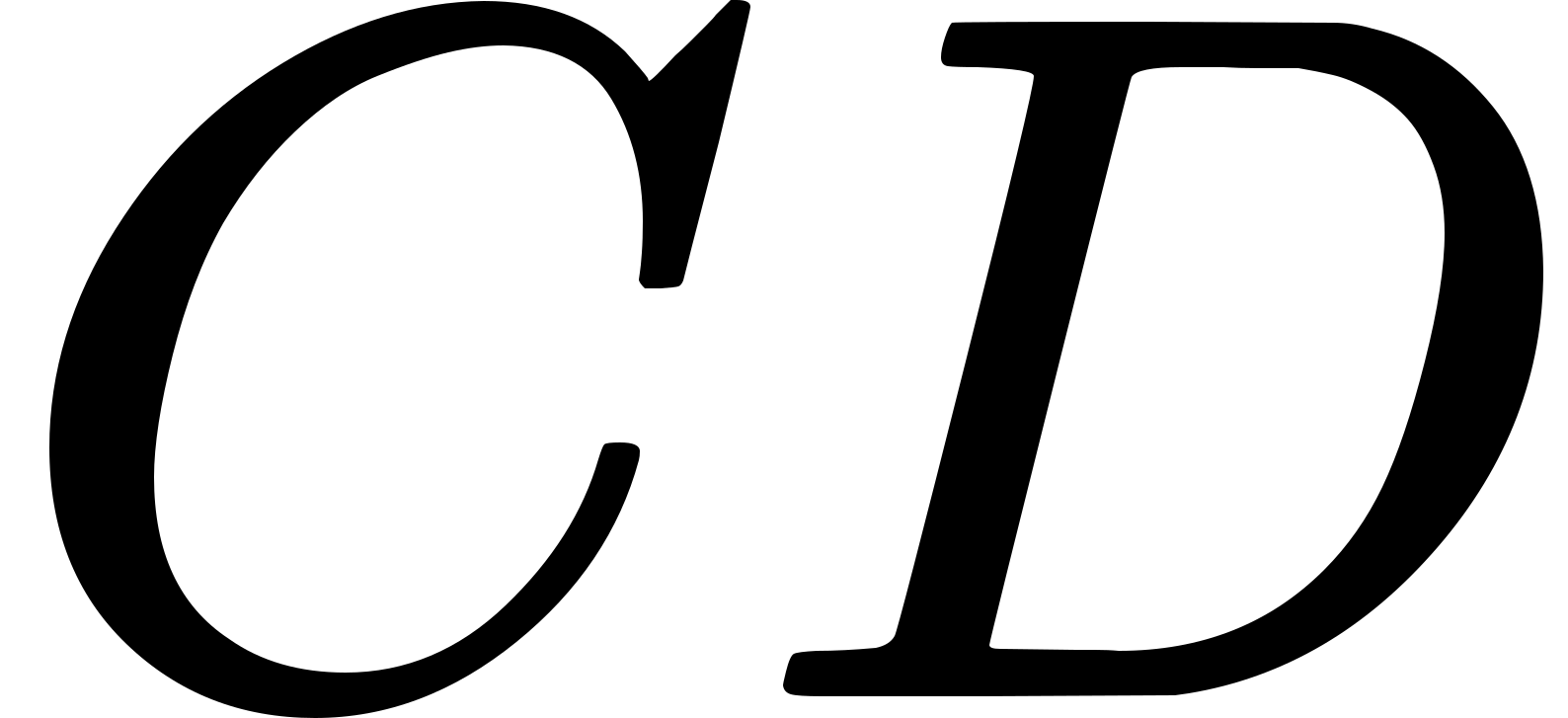 and
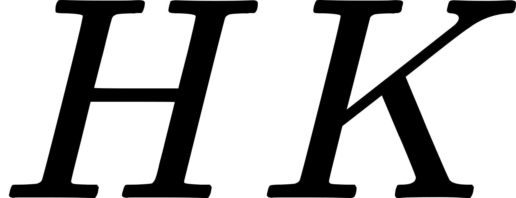
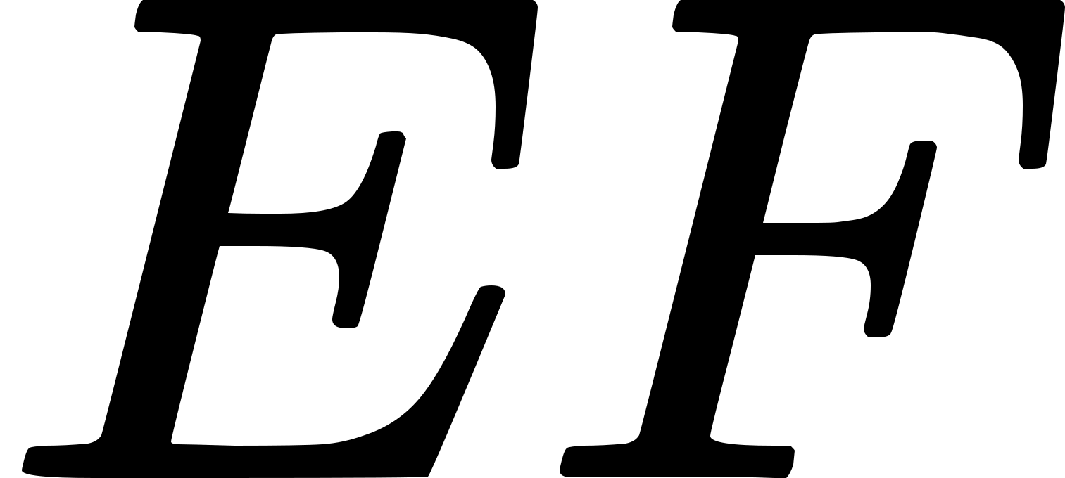 represents another duration which is extended over by the duration
bounded by
 . Two such durations
necessarily intersect and also can neither completely extend over the
other.
 of the same time-system when
 , then
 , say)
intersect in the levels
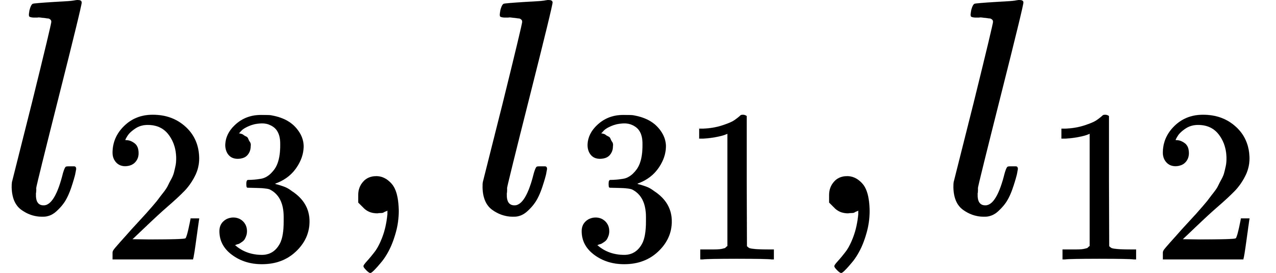 . Then
three cases can arise: either (i) the levels are all identical
[this will happen if any two are identical], or (ii) no pair of
the levels intersect, or (iii) a pair of the levels, say
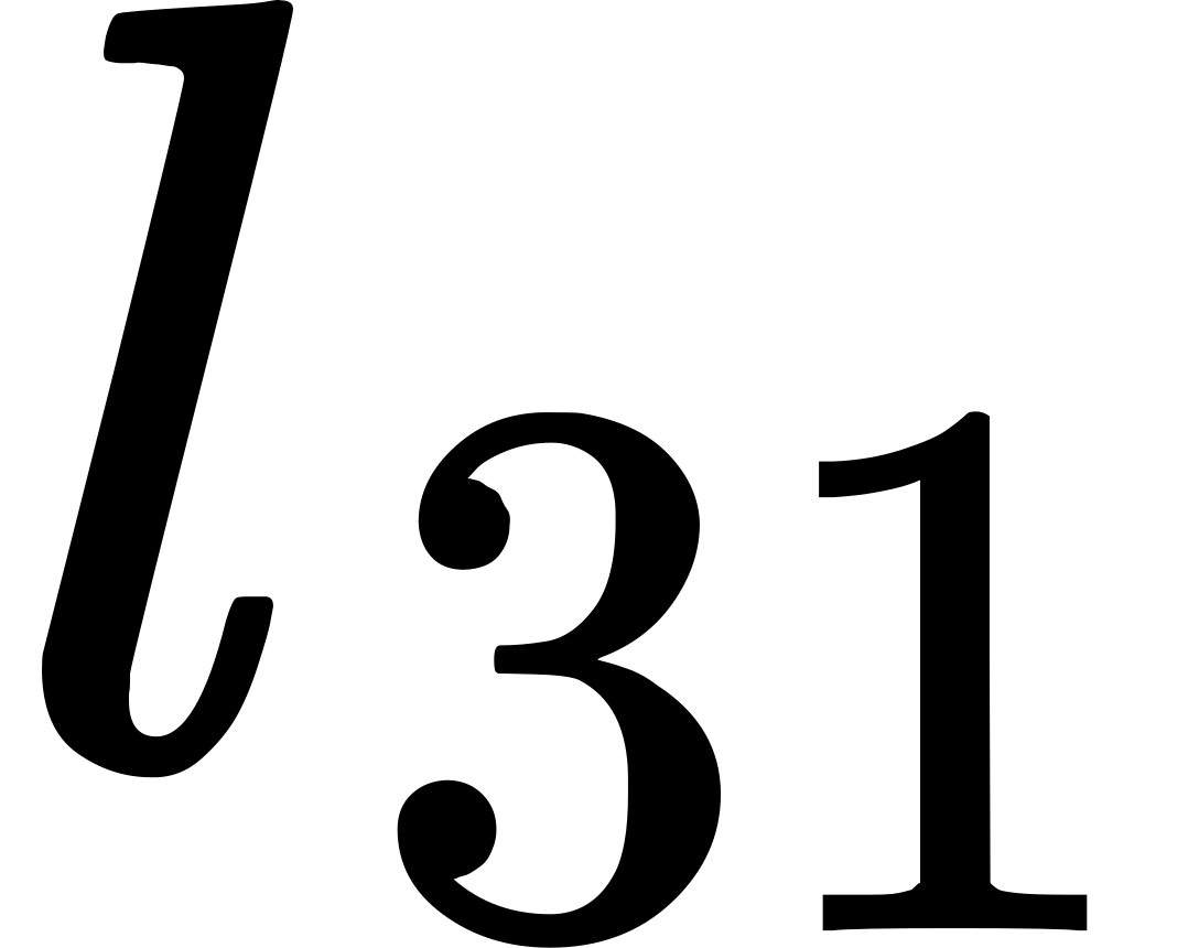 and
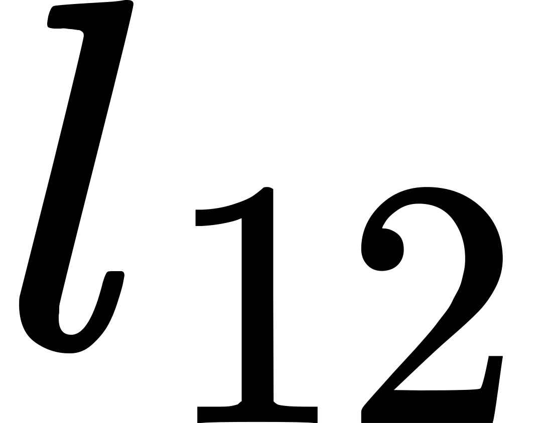 , intersect. In case (i) the three moments are
called 'co-level.' In case (ii) there are special relations of
parallelism of levels, to be considered later. In case (iii) the locus
of abstractive elements and abstractive classes which forms the
intersection of
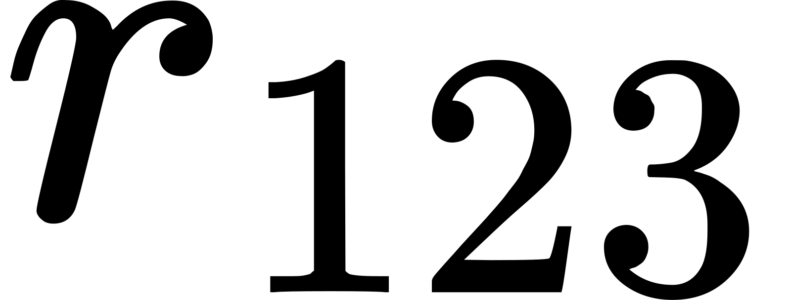 . Then
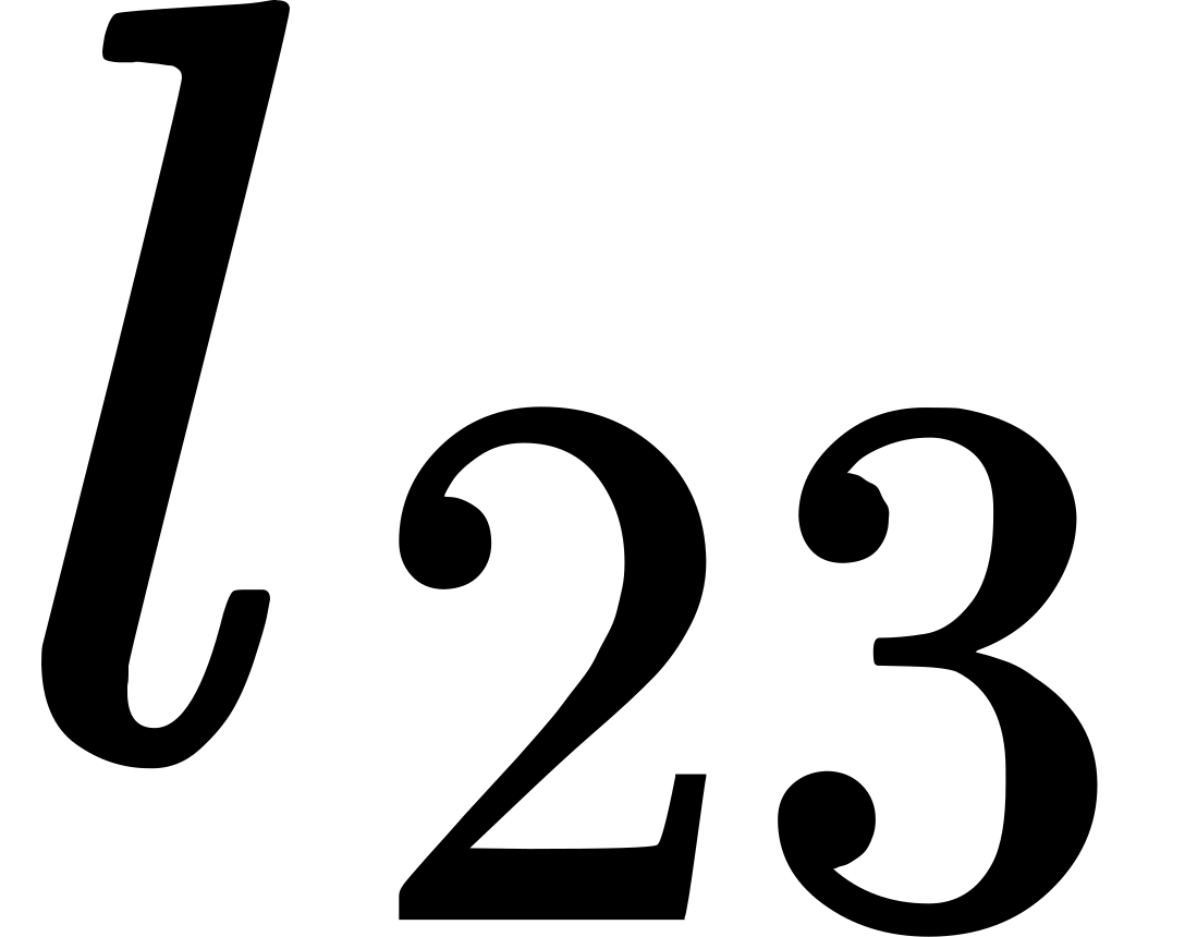 , and of and
 . When three moments have a
rect as their complete intersection they are called 'co-rect.' A rect is
an instantaneous straight line in the instantaneous three-dimensional
space of any moment in which it lies. But, as before, the conventional
space-nomenclature is avoided in connection with instantaneous spaces.
 which constitute an
instance of case (iv). Let
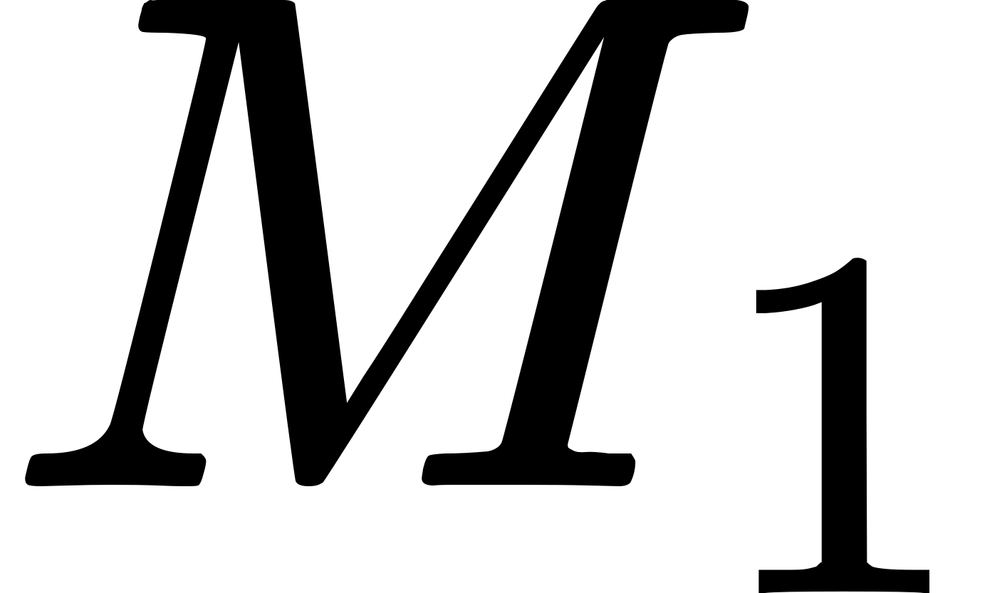 and
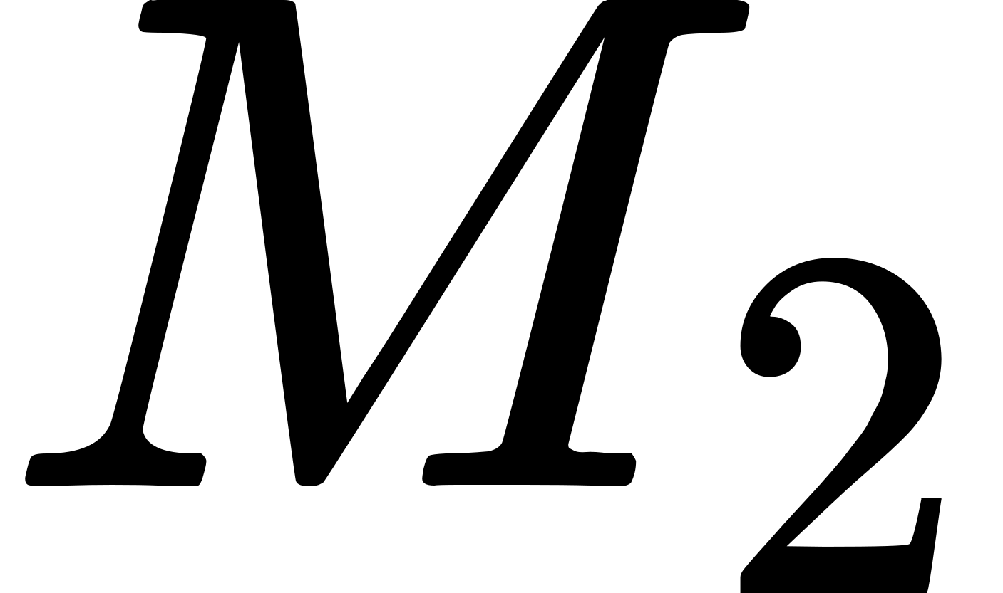 , and let be the rect which is
the intersection of
 . Then the rect
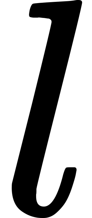
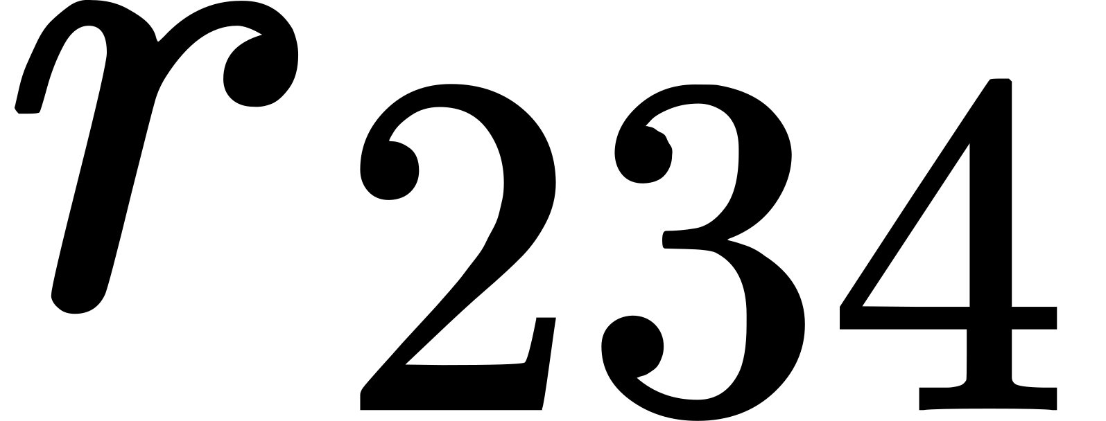 does not lie in the level
 and
 and
 and
 , and
 )
which (i) covers two event-particles
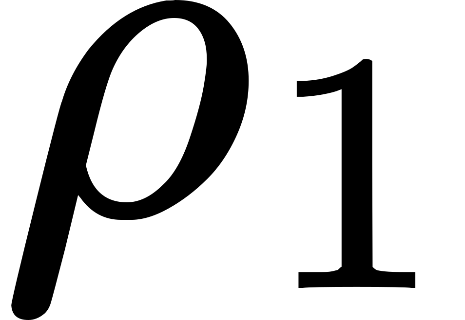 and
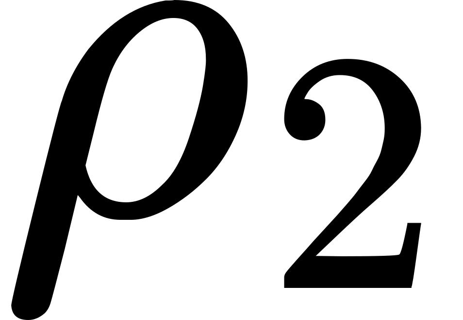 (called the end-points), and (ii) is such that no selection of the
event-particles which it covers can be the complete set of event-particles
covered by another simple abstractive class, provided that the selection
comprises
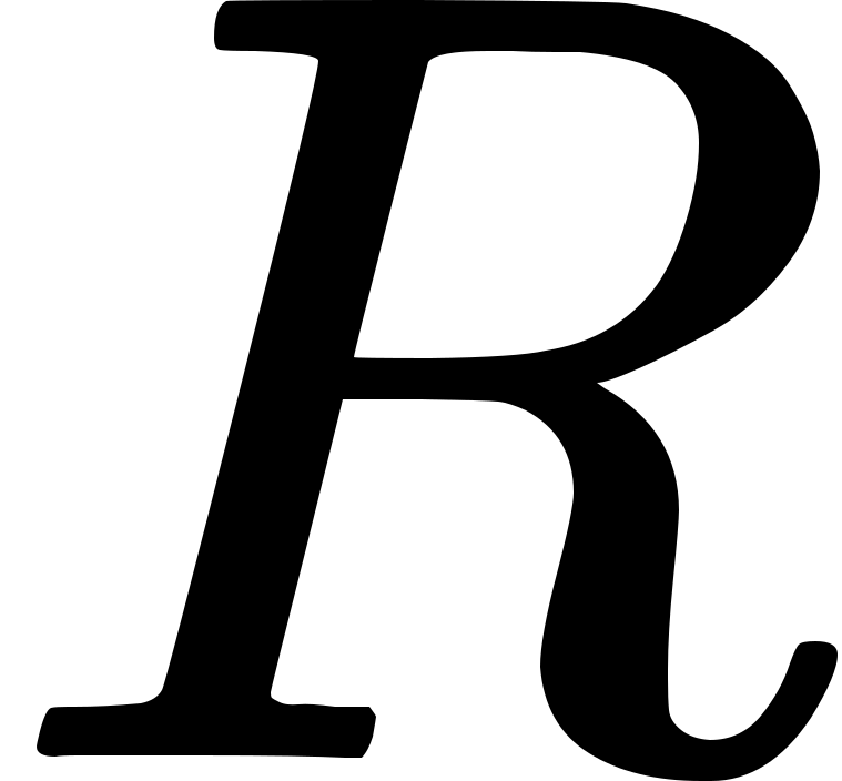 ,
there is one and only one route with
 ,' and let '
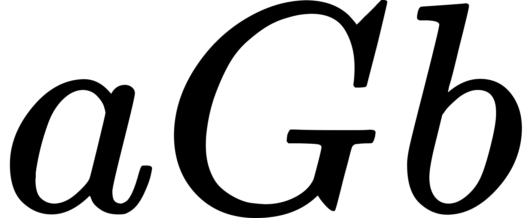 ' mean '
 and
 be any other duration of the same time-system
which intersects
 (say), which covers
 , and let
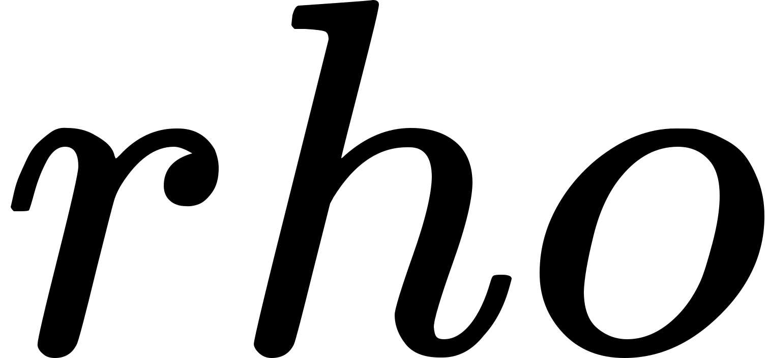 be any complete family of parallel rects. Then a certain
set of rects belonging to
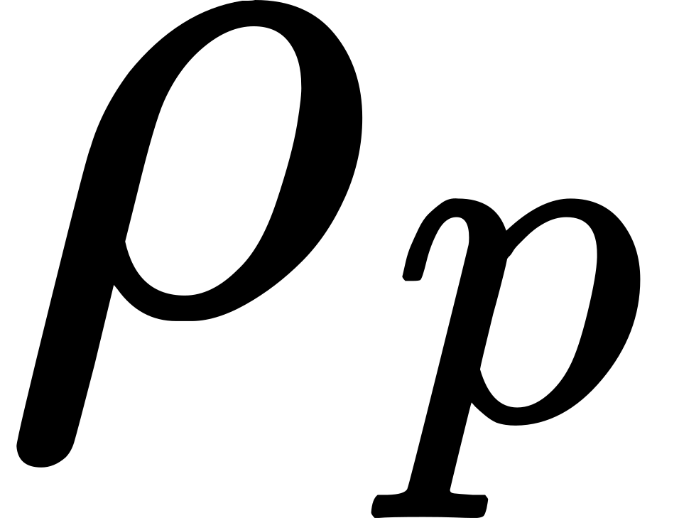
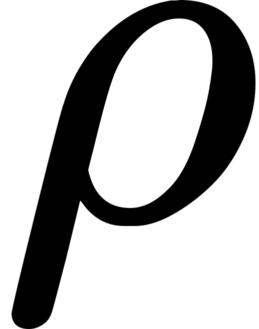 will intersect
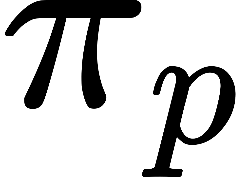
 . Let
 . Let P be
any event-particle occupying some member of
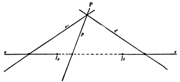
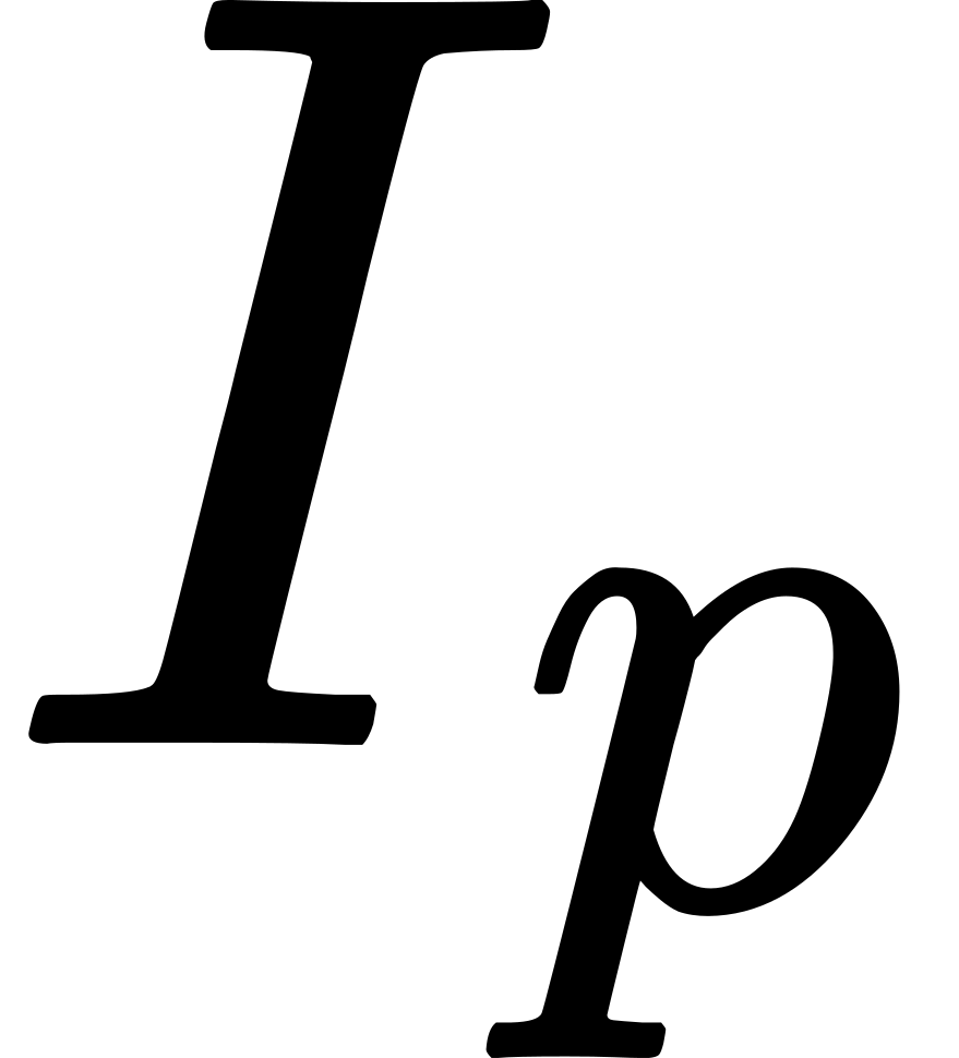 and
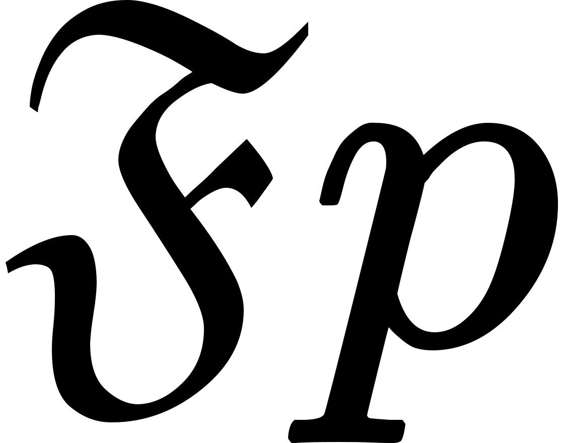 . The
segment between
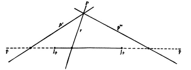
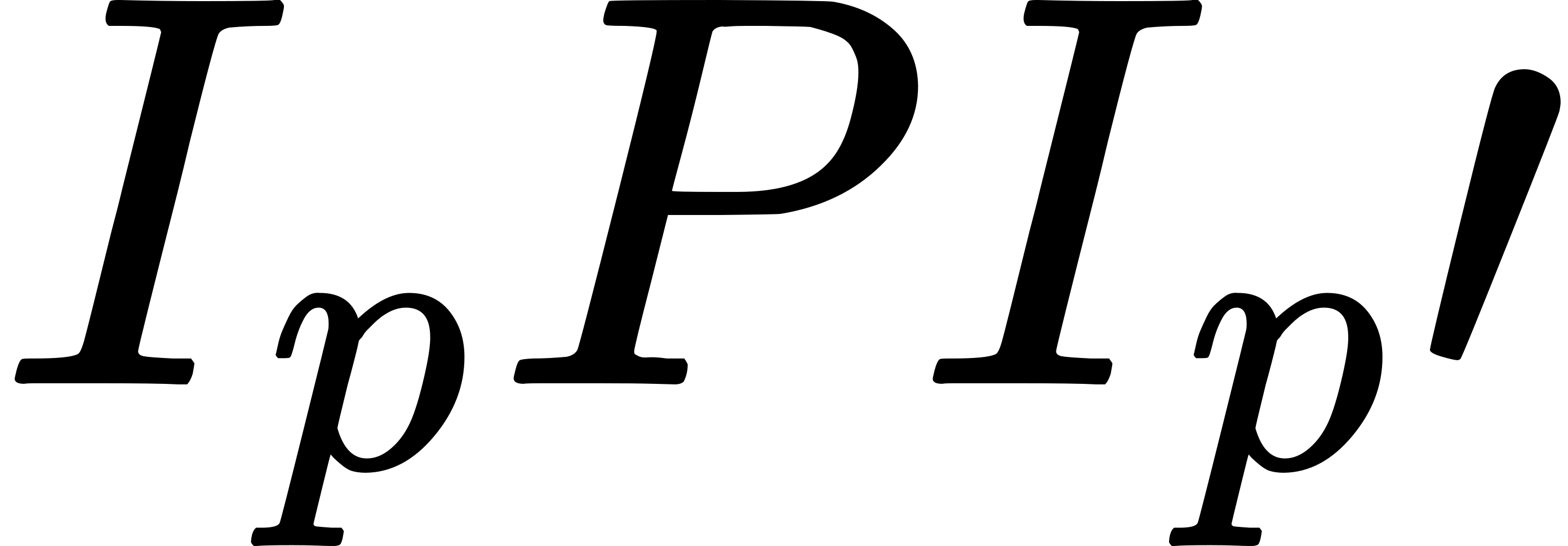 and
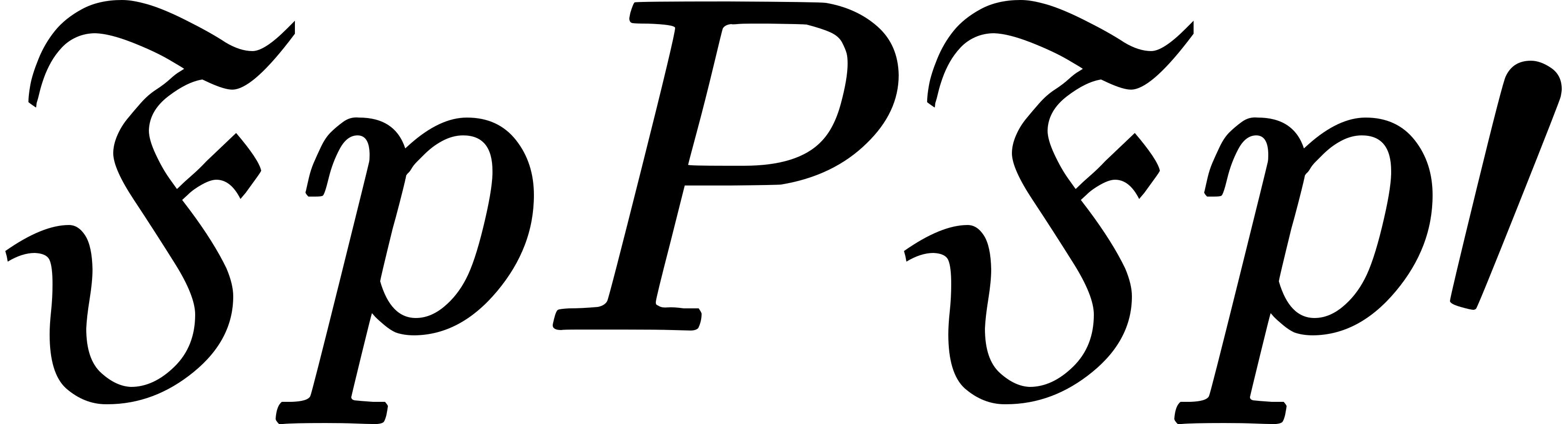 which may equally well be termed rects or point-tracks.
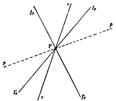
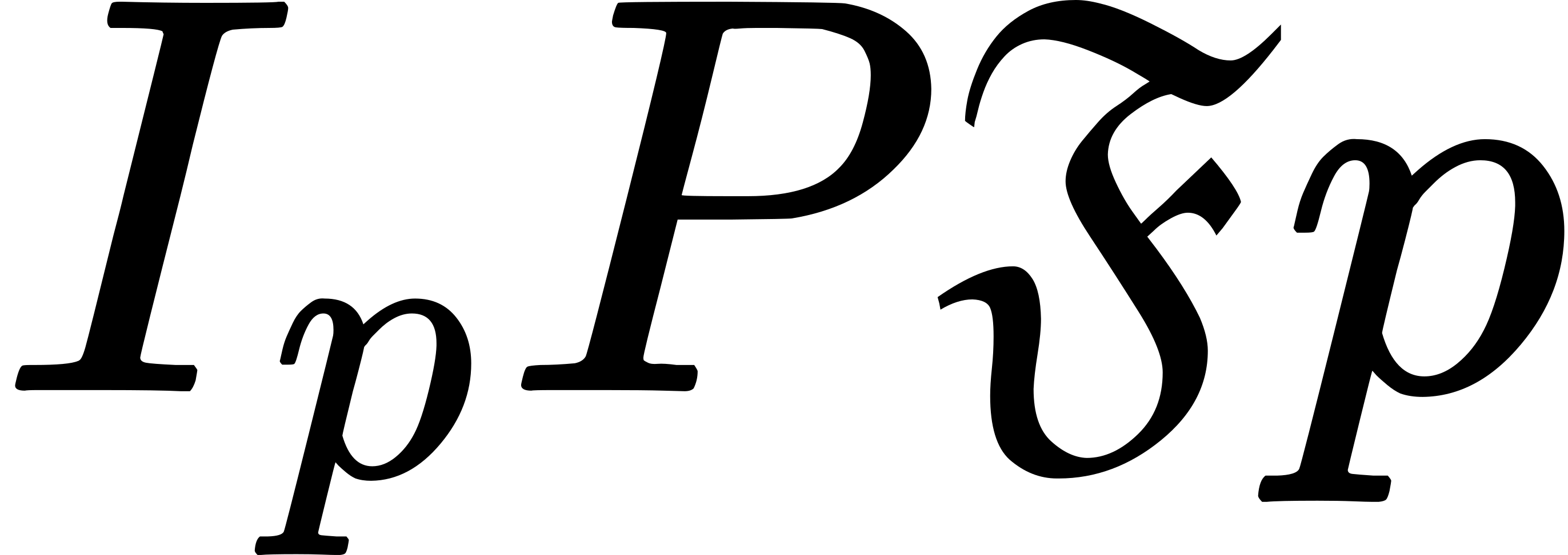 and
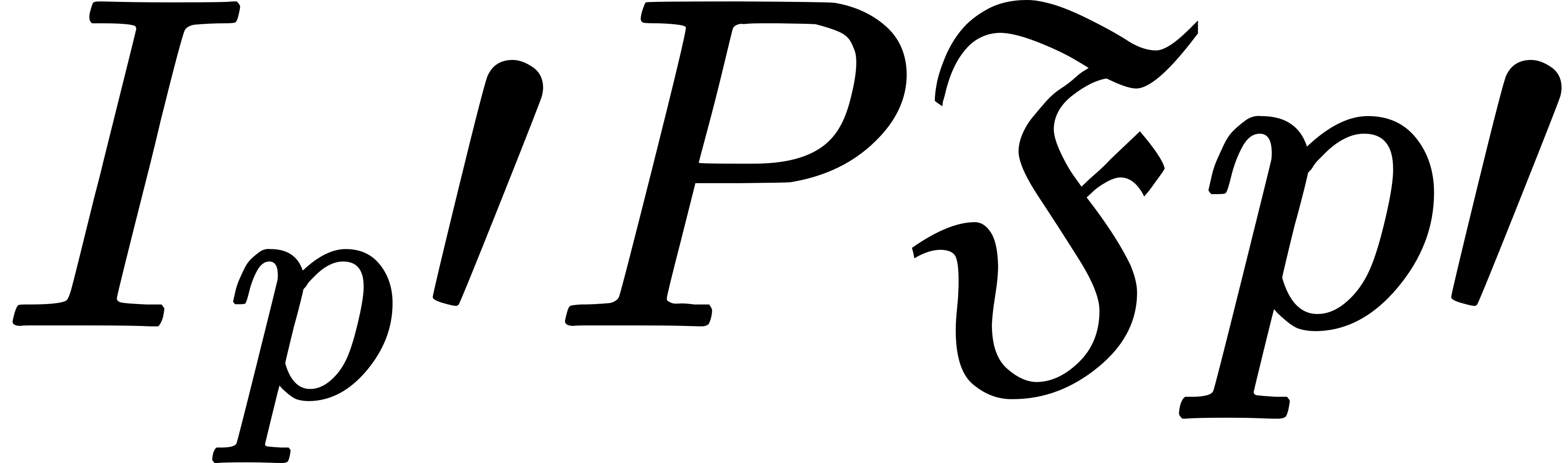 are joined to
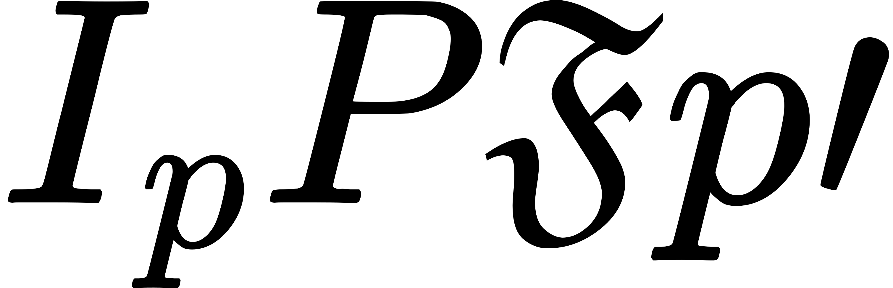 and
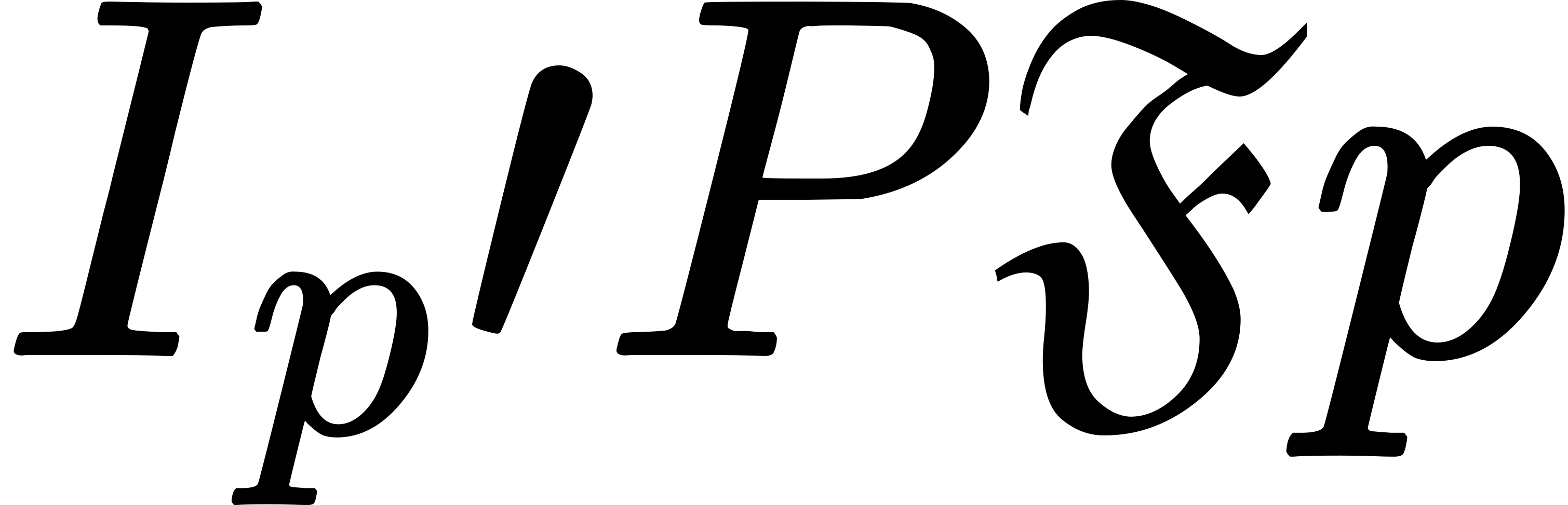 are joined to
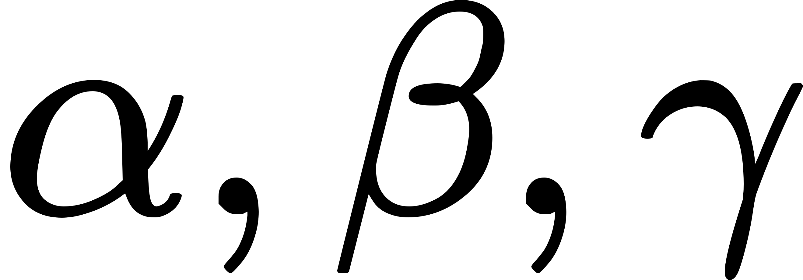 , ... be the collinear set of time-systems
whose points lie in or are parallel to the matrix
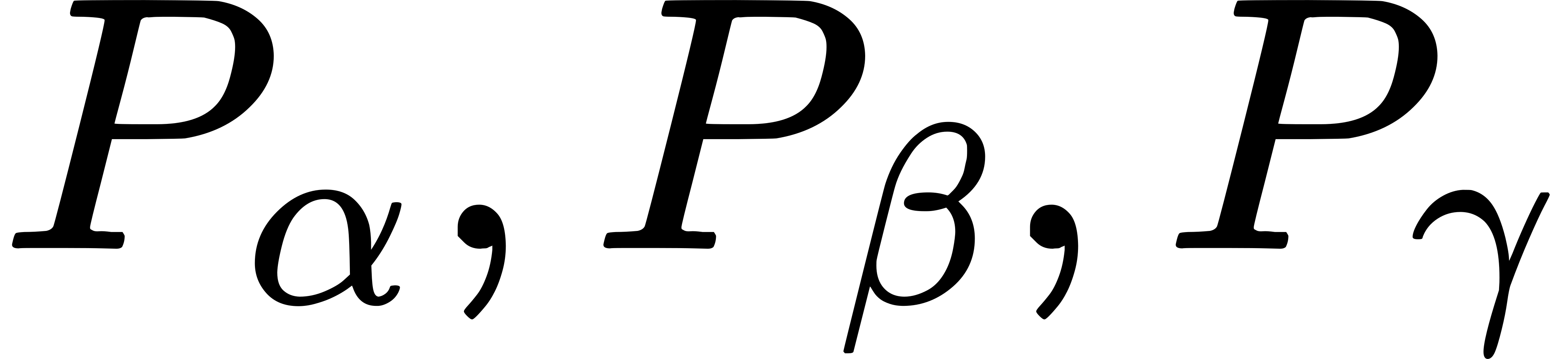 , ... be the moments of the
time-systems
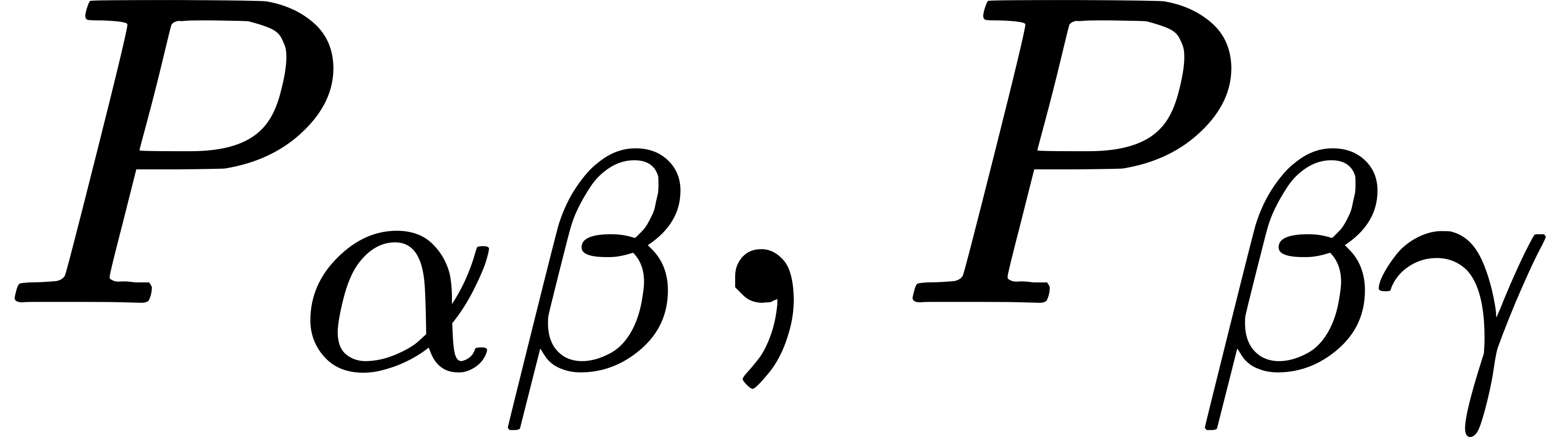 , ... in which respectively
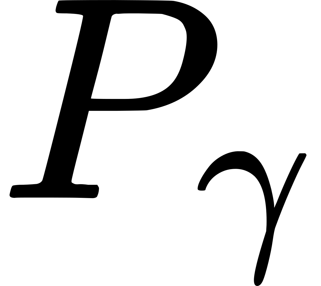 ,
etc., intersect are identical, and the event-particle
 , etc., respectively.
The level
 , etc., of the spaces of
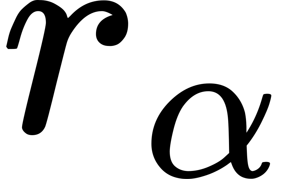 contains
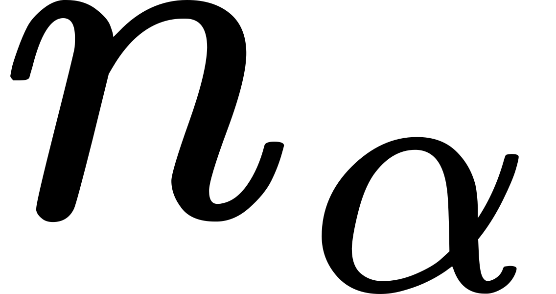 and
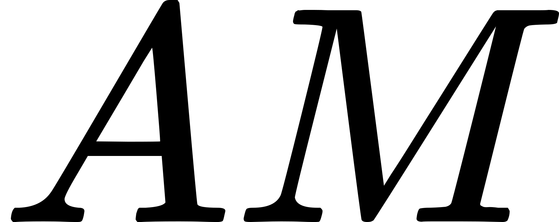 and
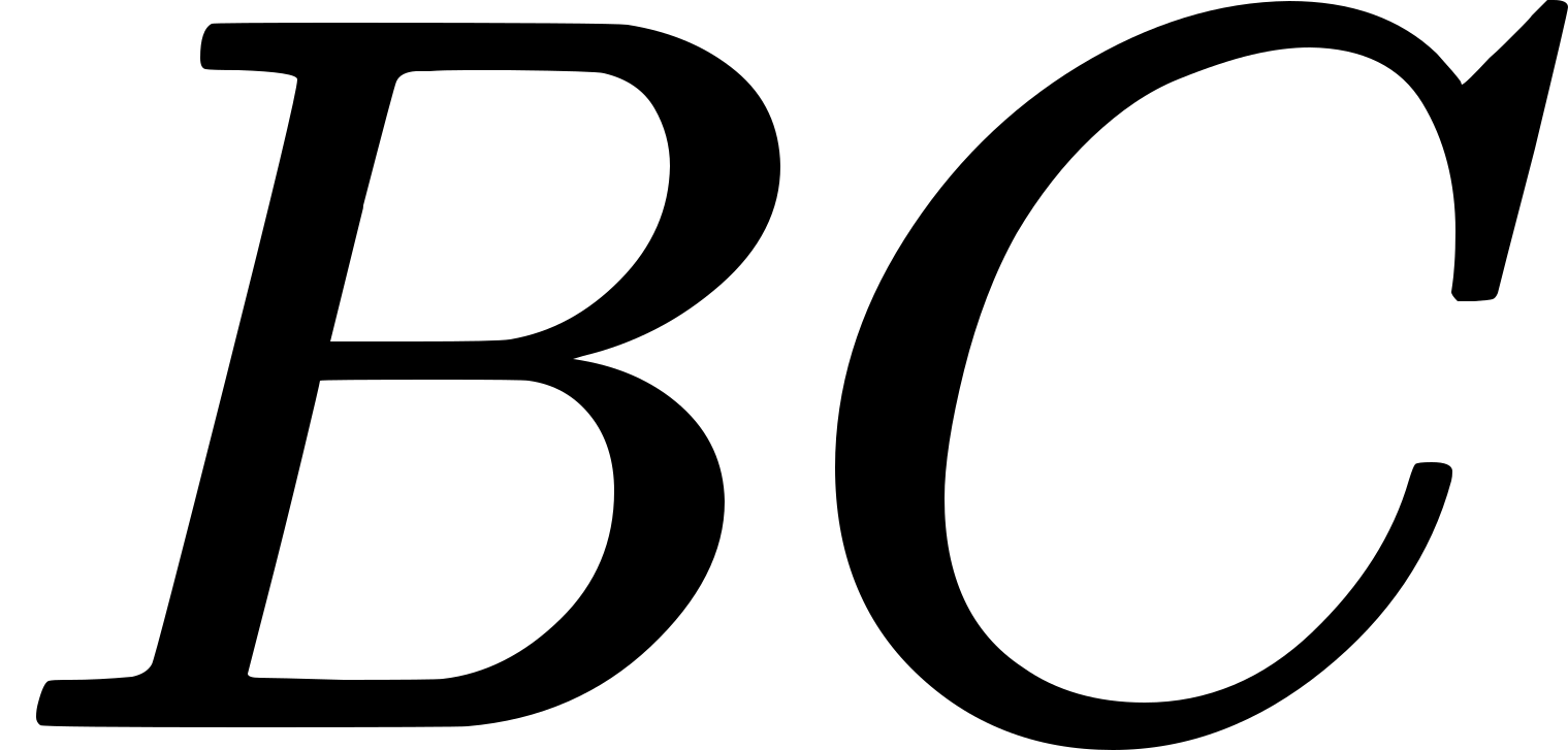 be a pair
of mutually normal rects intersecting at
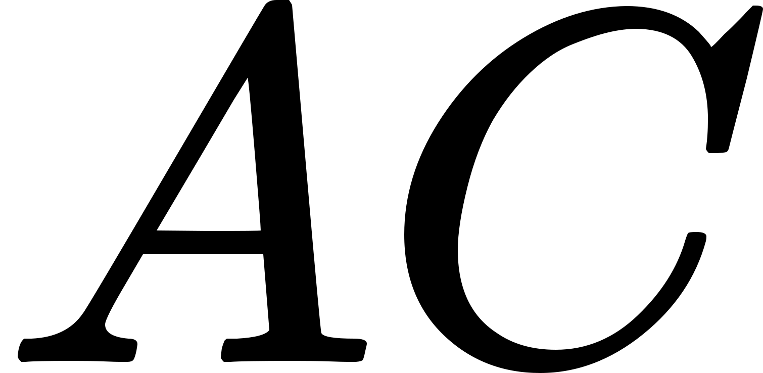 are congruent to
each other.
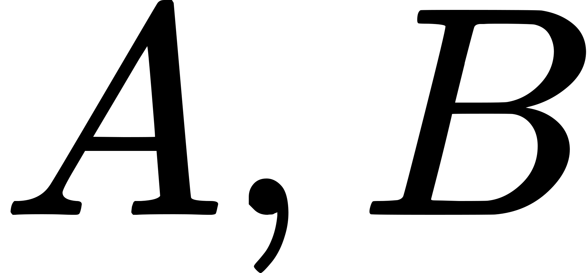 ) and (
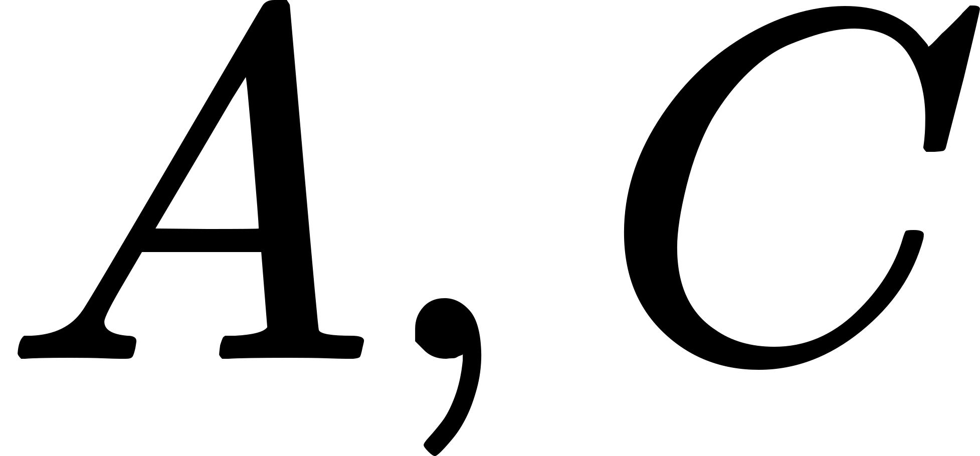 ), are joined by rects, or both pairs are joined
by point-tracks, or both pairs by null-tracks. As in the analogous case
of congruence derived from parallelism, the transitiveness of congruence
expresses a substantial law of nature and not a mere deduction from the
terms of the definition.
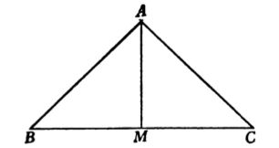
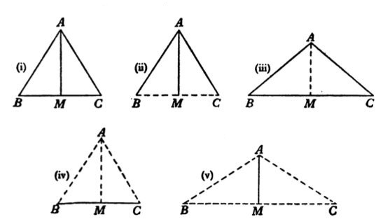
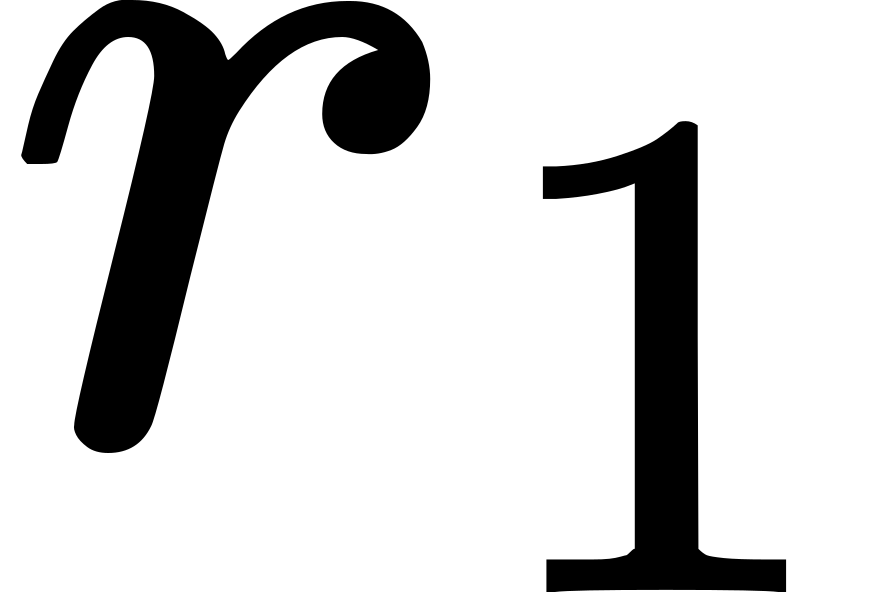 and
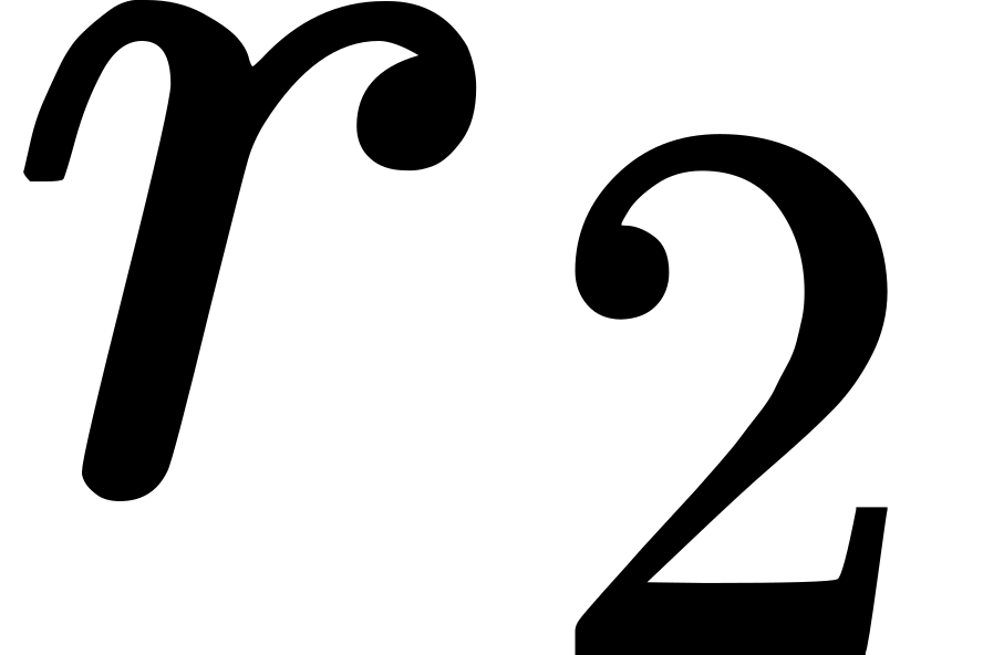 be any two co-momental rects intersecting in
the event-particle
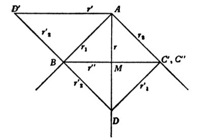
 . Through
 and
 .
Thus
 . Hence by case (i) of
 . Thus lengths on
 apart from the assumption
of the theorem which we want to prove.
 ) form a sort of 'material'
objects when (i) the objects of the set
 which is a section of
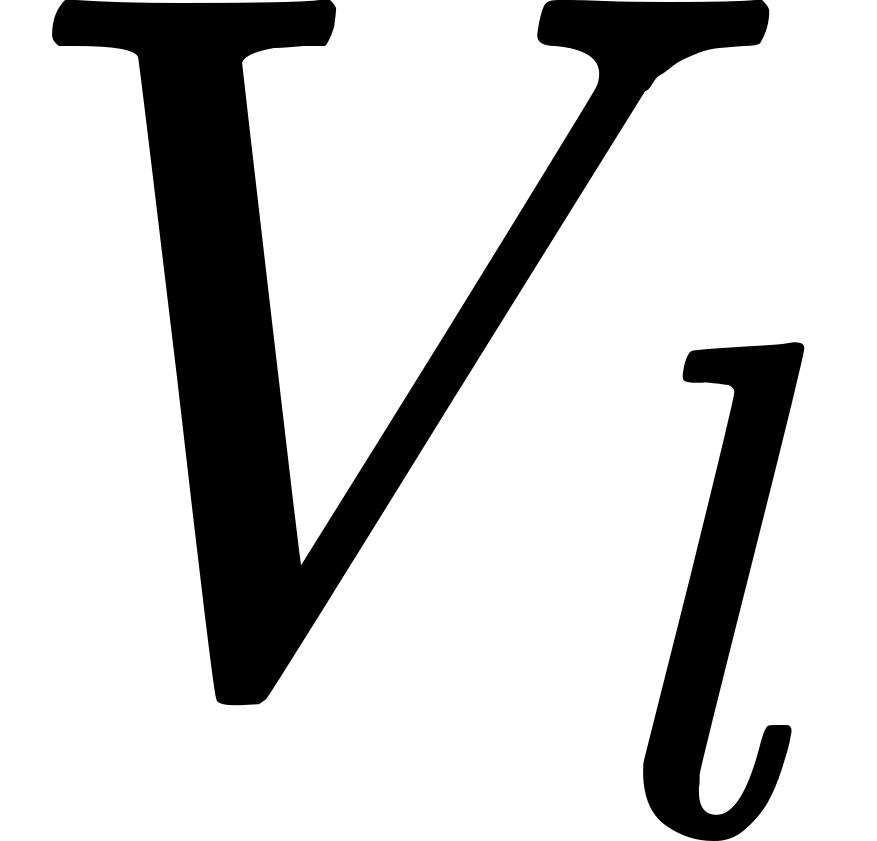 be any volume which is a portion of
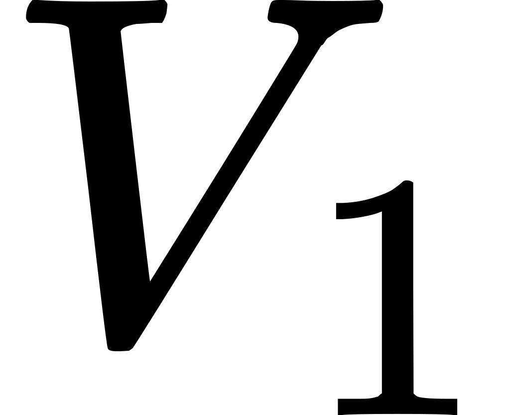 and is a concurrent component of
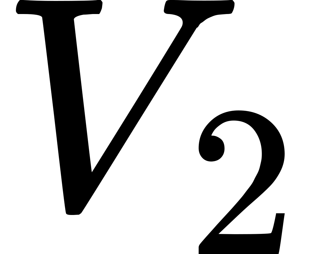 which are geometrical
replicas of
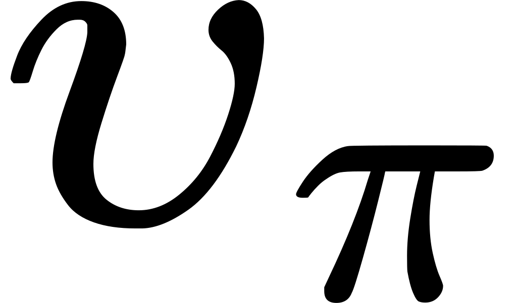 be the measure of the normal cross-sections of
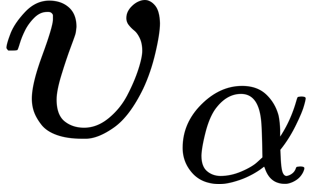 be the measure of the oblique cross-sections made
by moments of
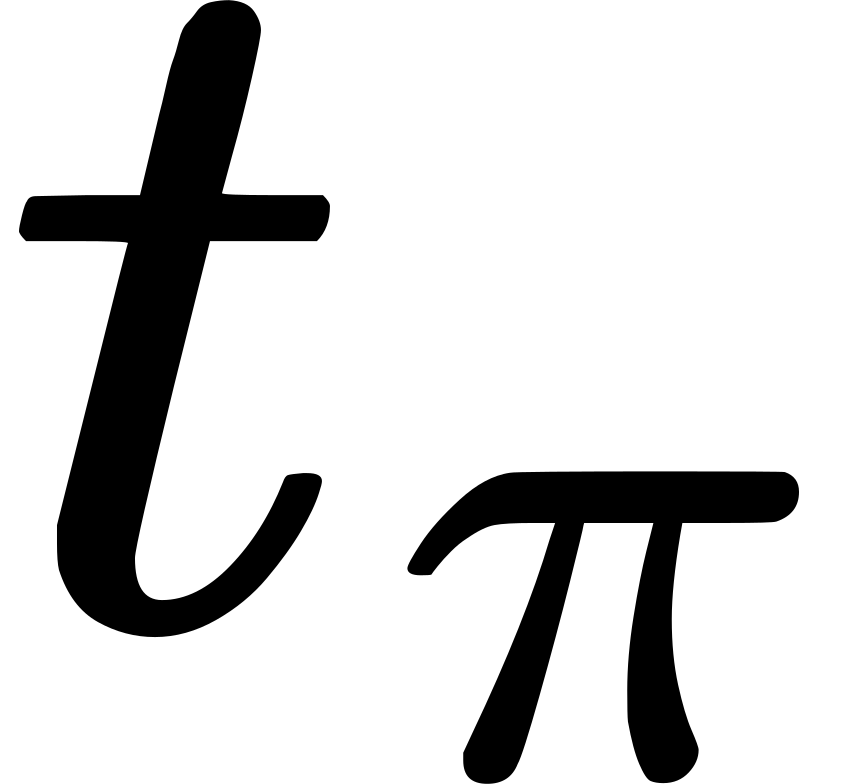 . Then if (
 )
be the
 )
be the



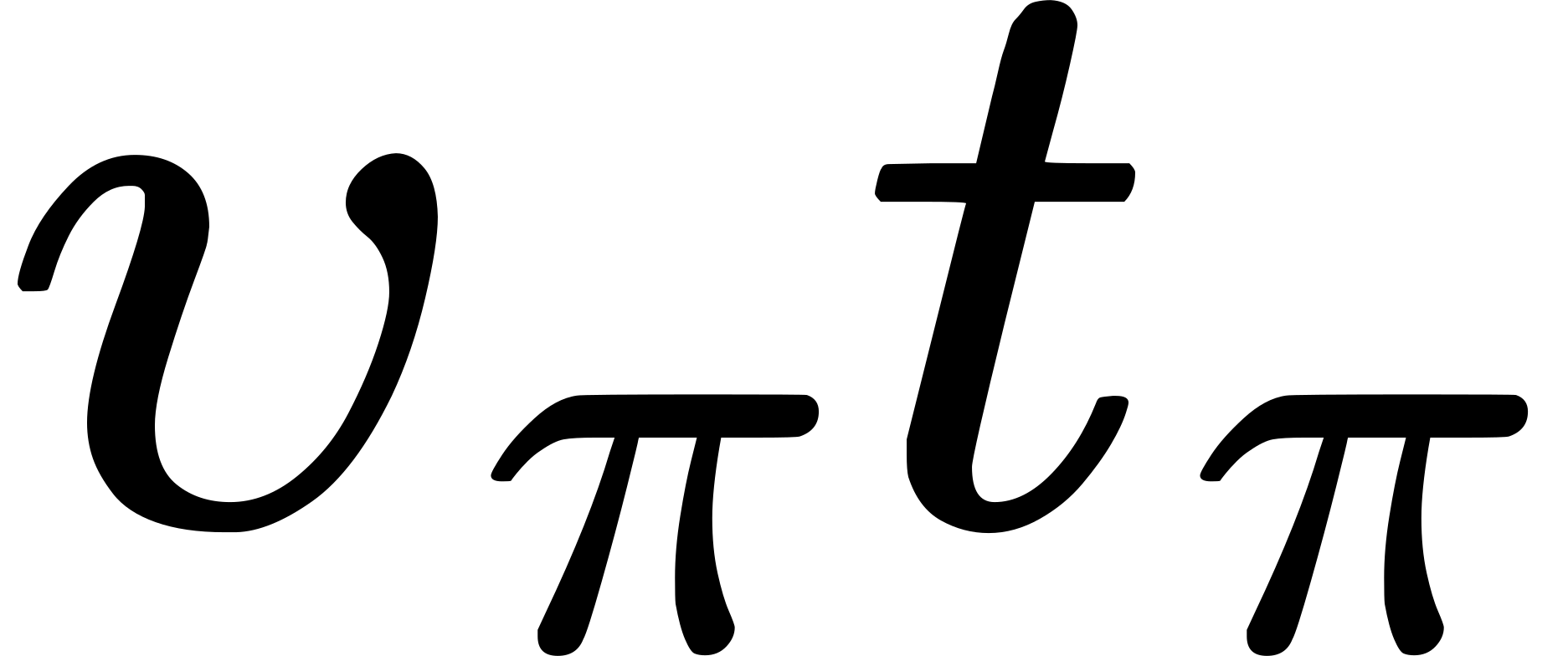 and as
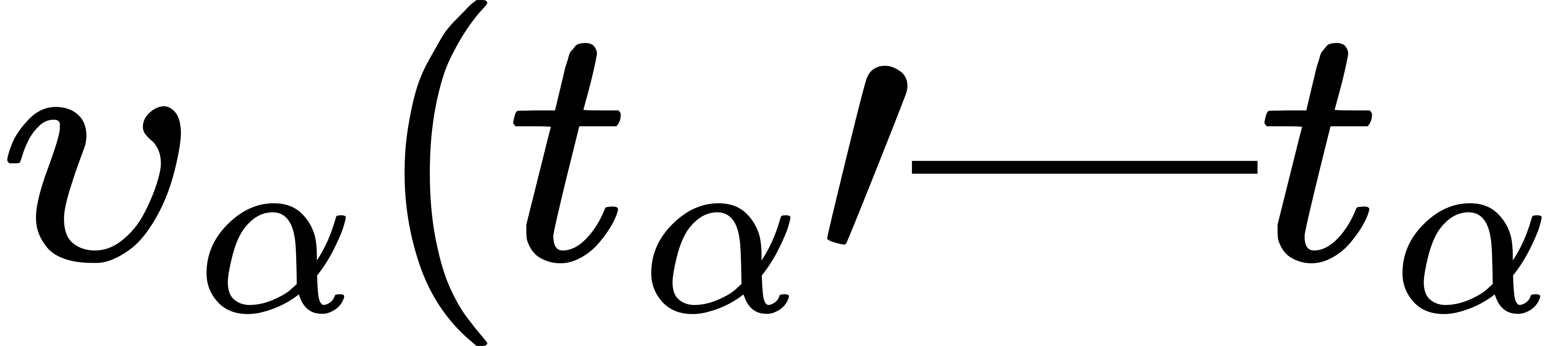 ). Hence
 .

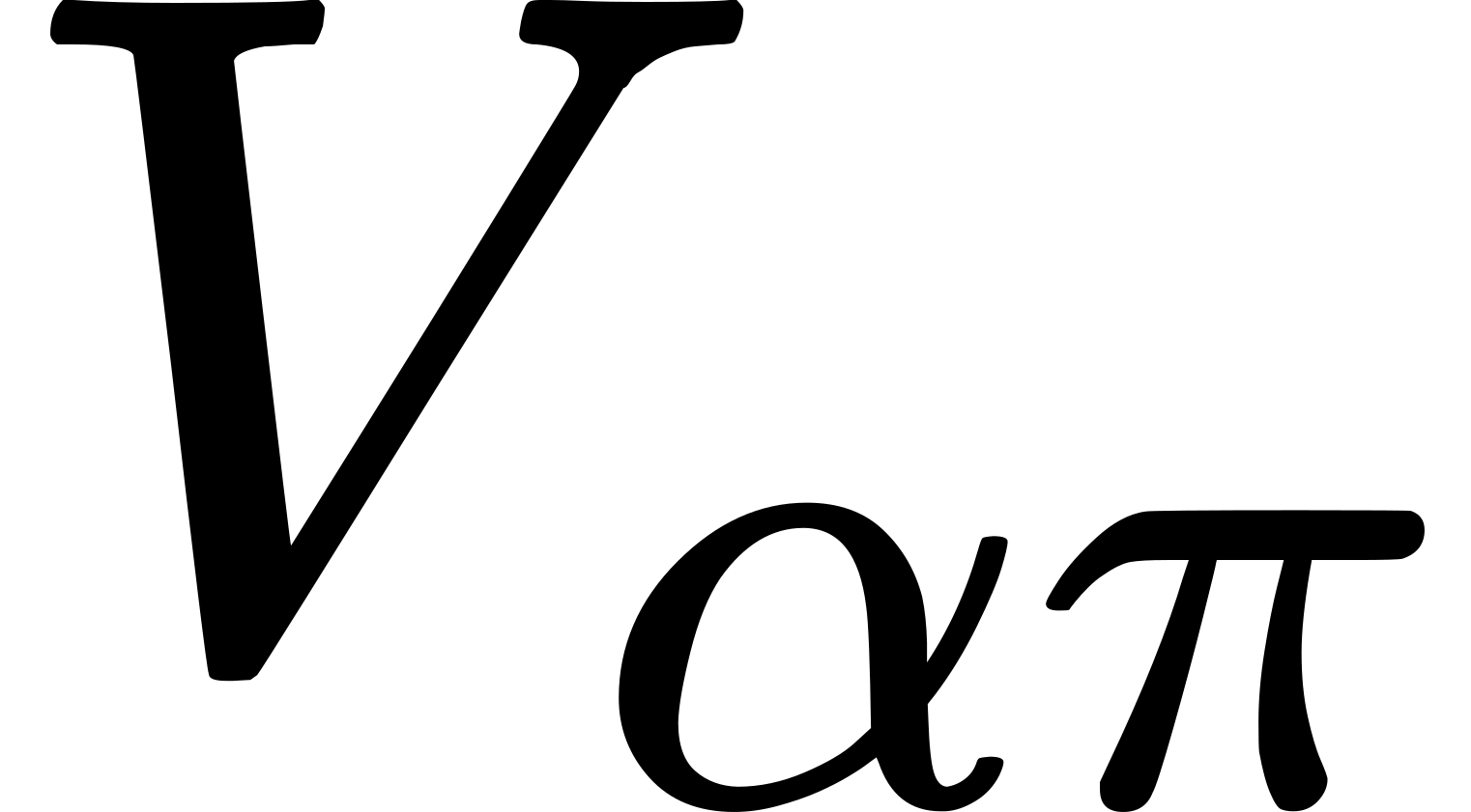 , namely the velocity due to
the time-system
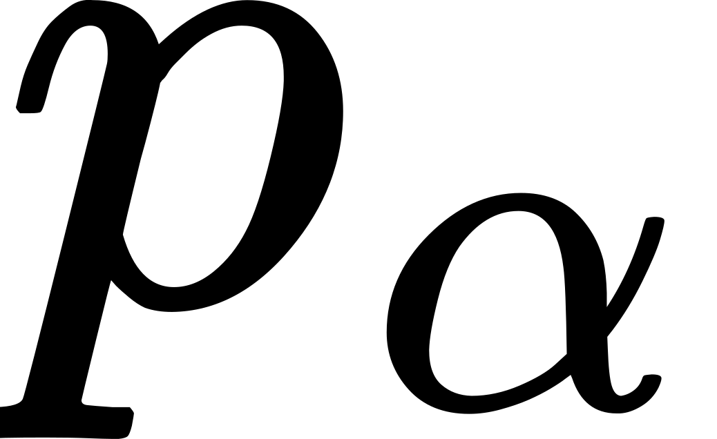 at the
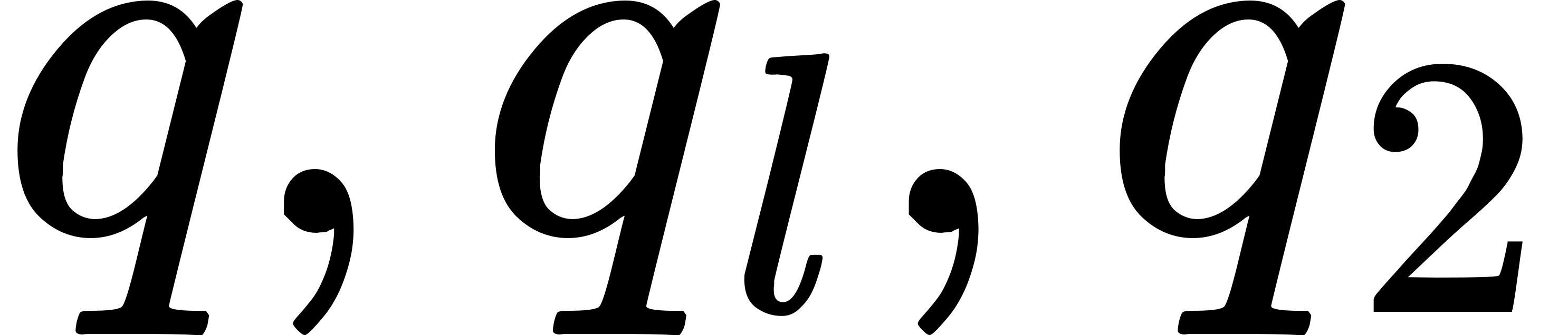 being the quantities possessed respectively by
 ], then the kind of
quantity will be called 'absolutely' extensive. When an extensive
quantity is not absolutely extensive, it will be called 'semi-extensive.'
 . Then the electromagnetic mass of
the whole sphere is not the sum of the electromagnetic masses of these
two parts, but is to be calculated by a quadratic law from the charges.
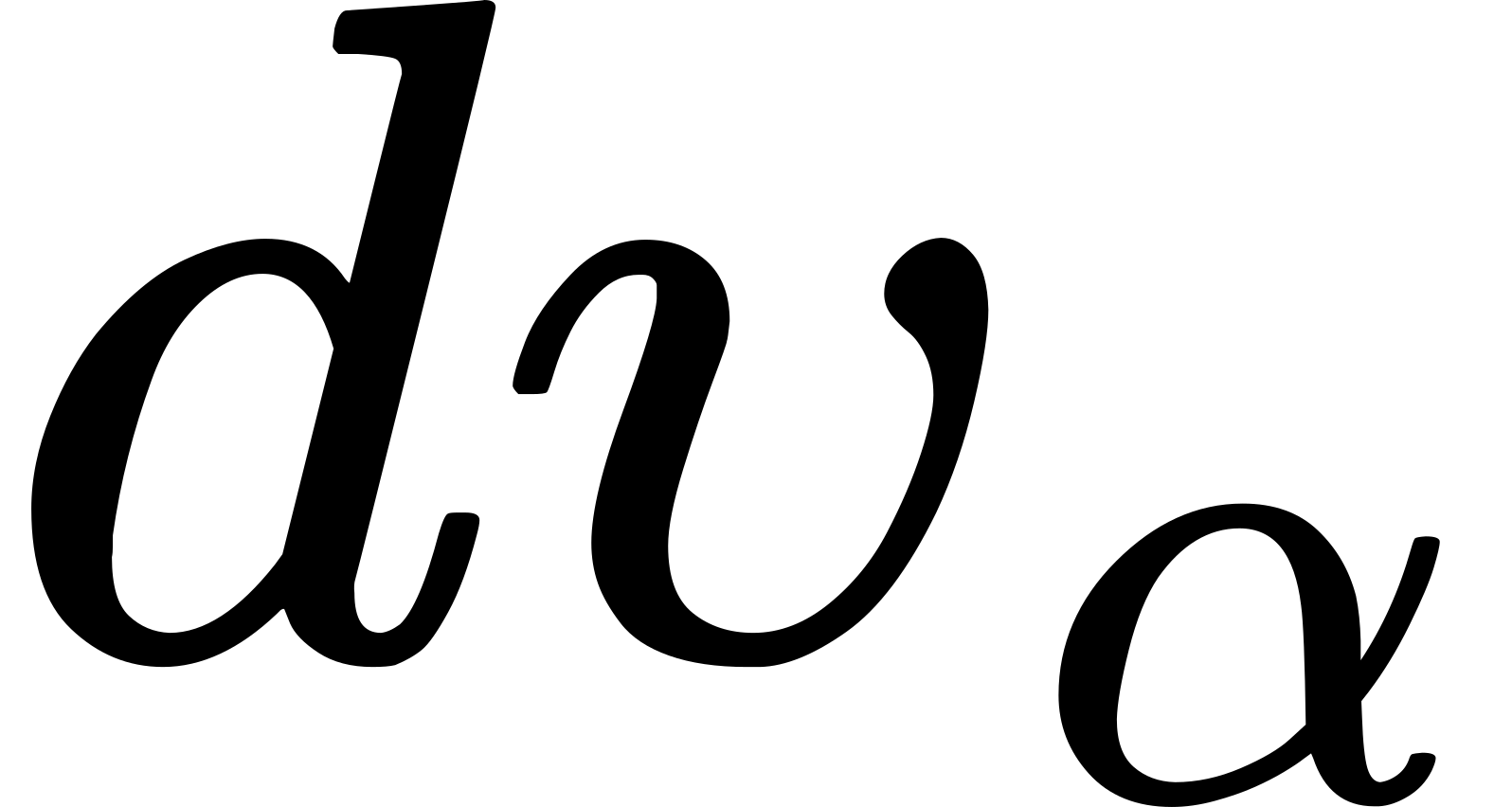 be the
measure of a volume in the
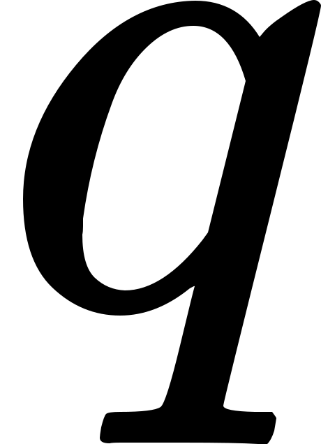 be the measure of the quantity possessed by
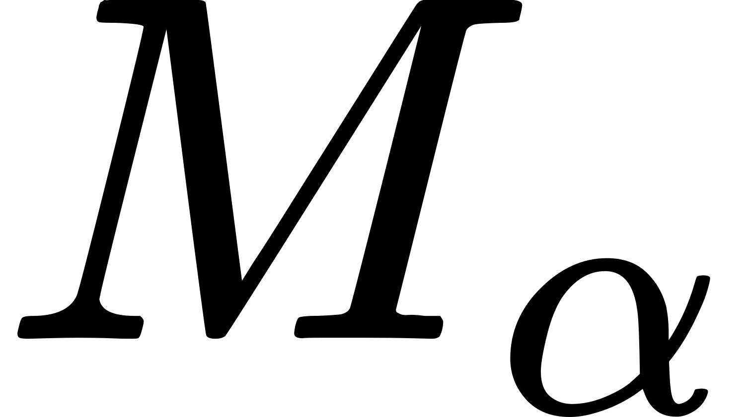 [i.e. at a time
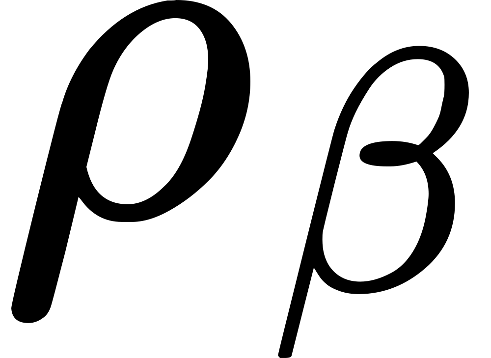 of an absolutely extensive
quantity for two time-systems
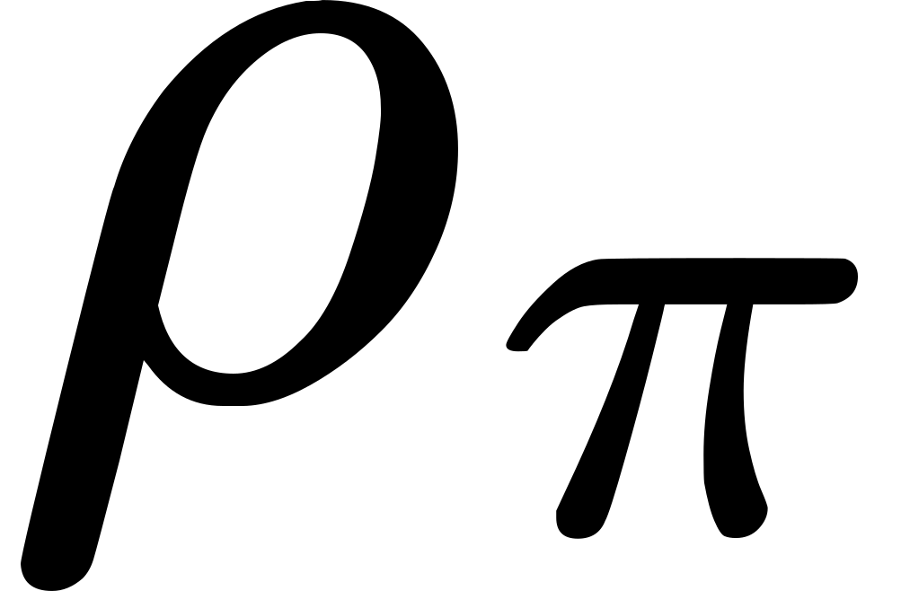 be the volume-density at
 be the
moments in
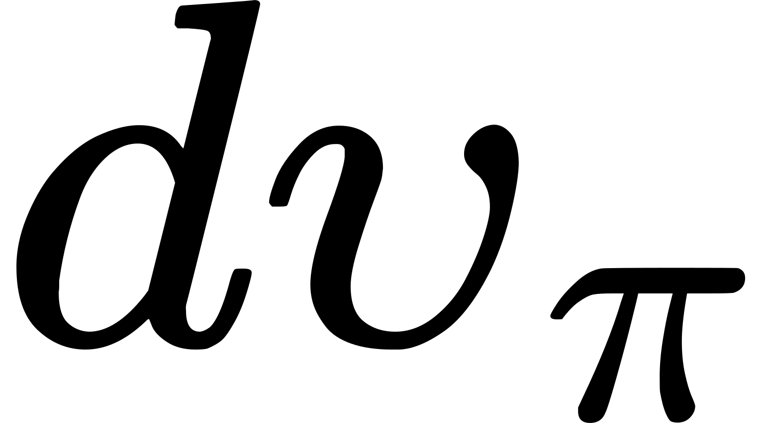 be the measure of a small volume in
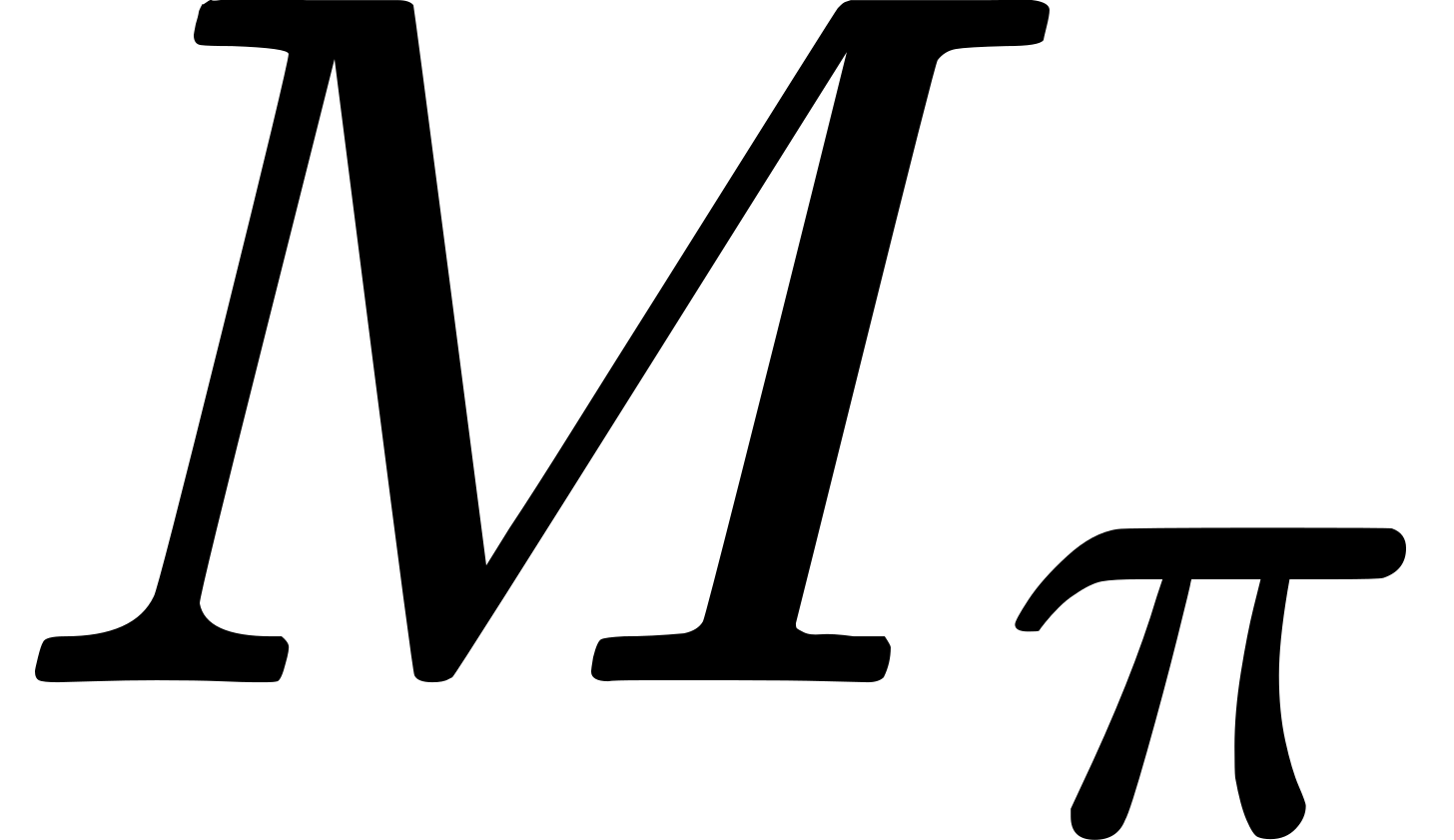 which contains
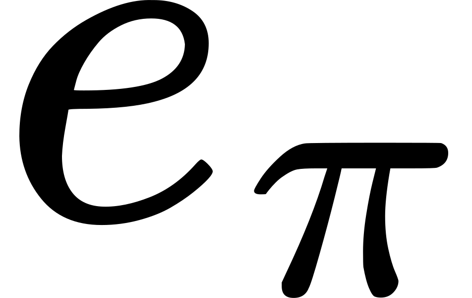 ) stationary in
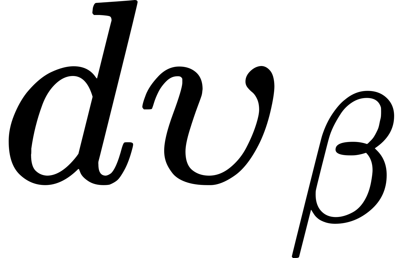 be the
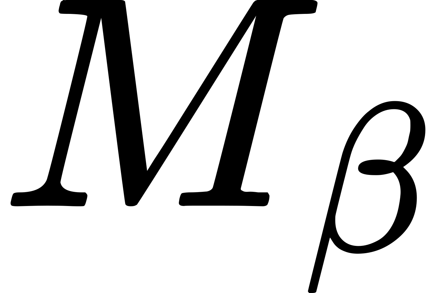
measures of the volumes which are the oblique cross-sections of
 . Then ultimately
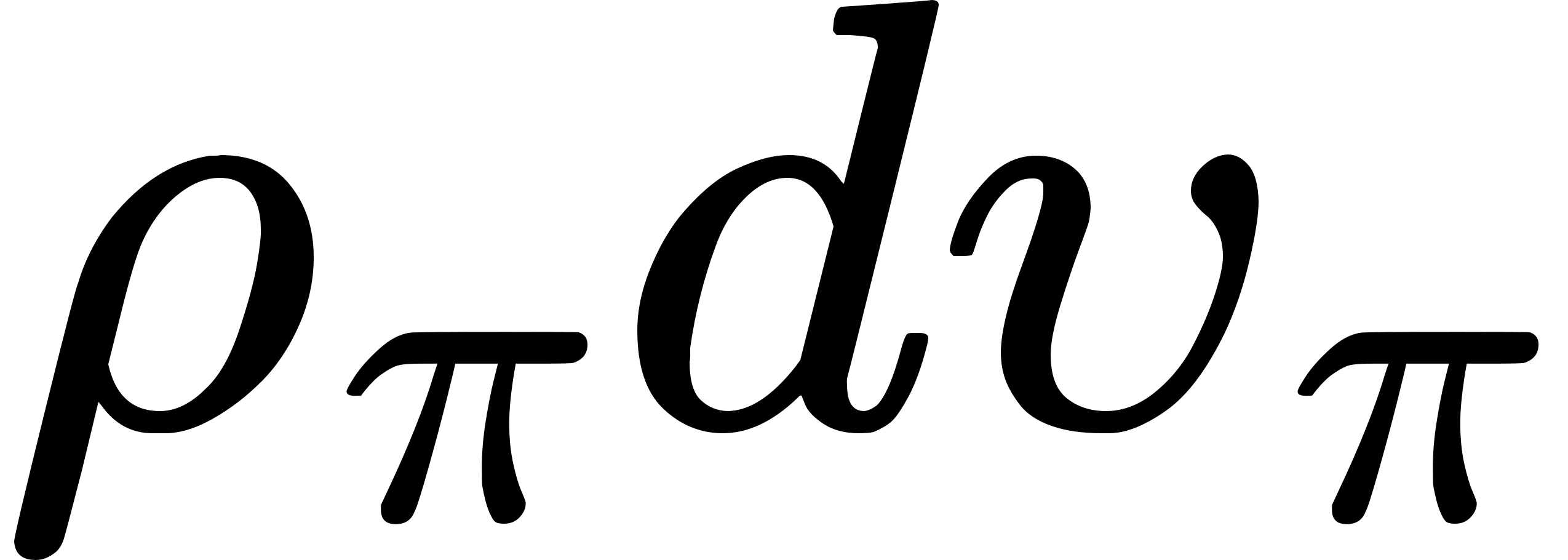 ,
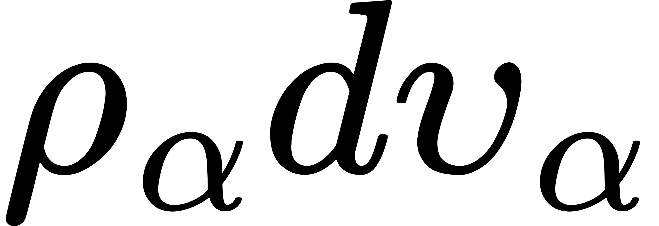 , and
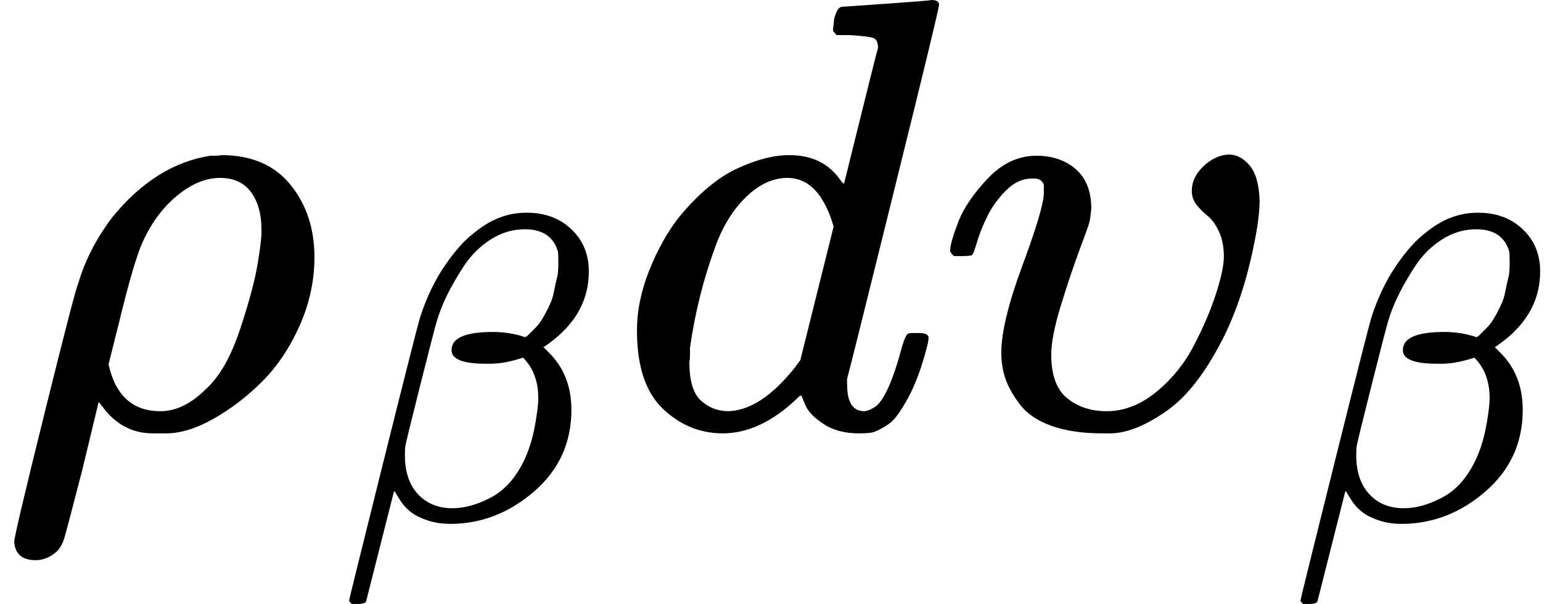 are expressions for the measure of the
quantity possessed by




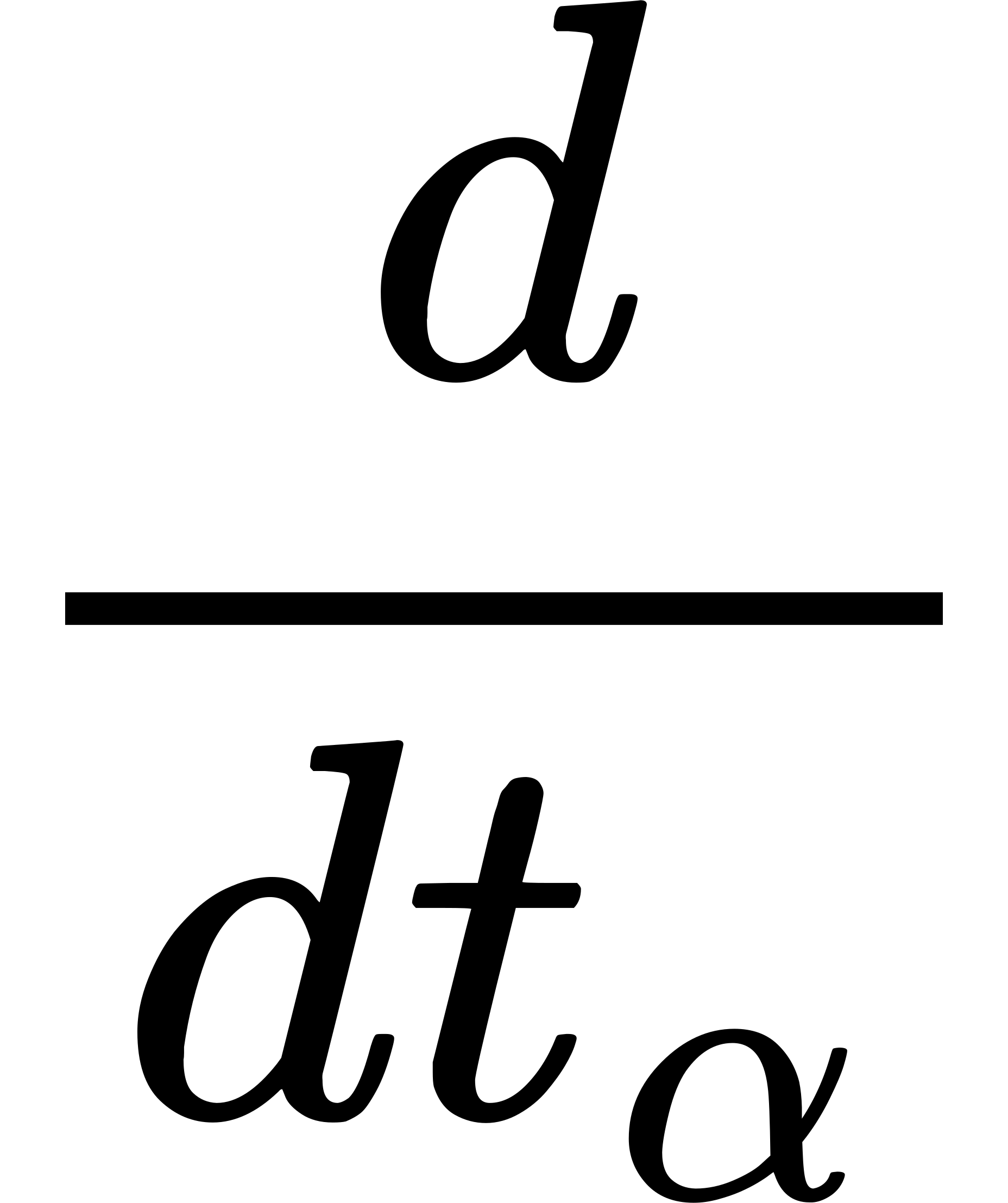 denote differentiation
following the motion
(
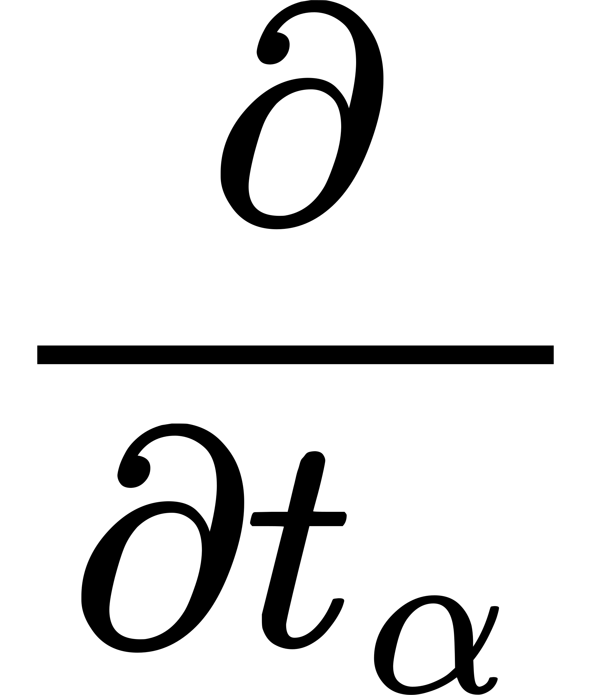 denote
differentiation at the point (






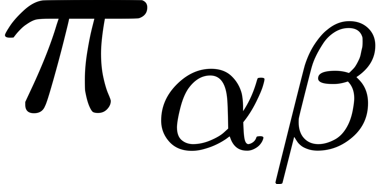 which lies in the instantaneous three-dimensional
moments
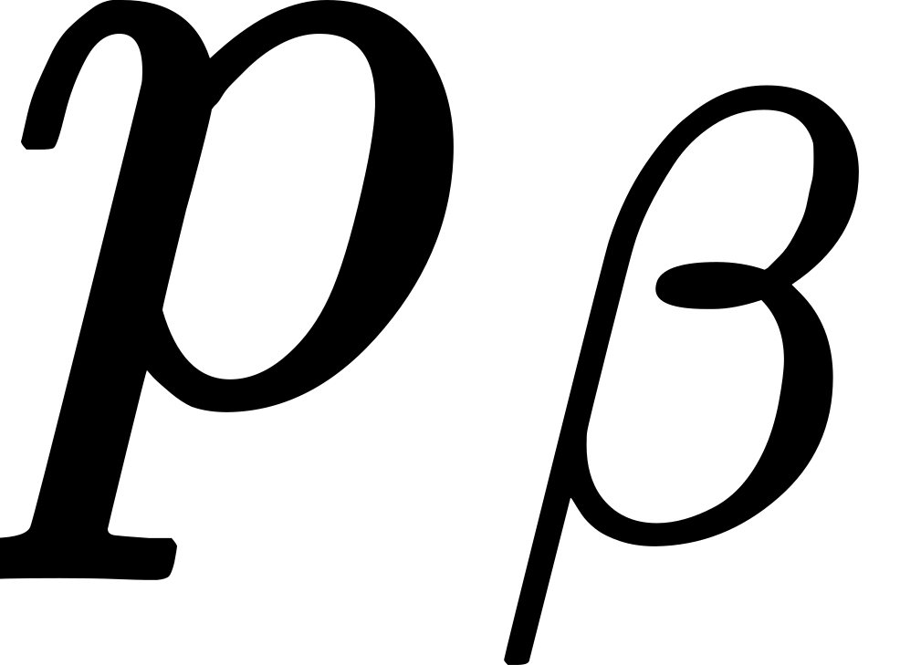 belonging to
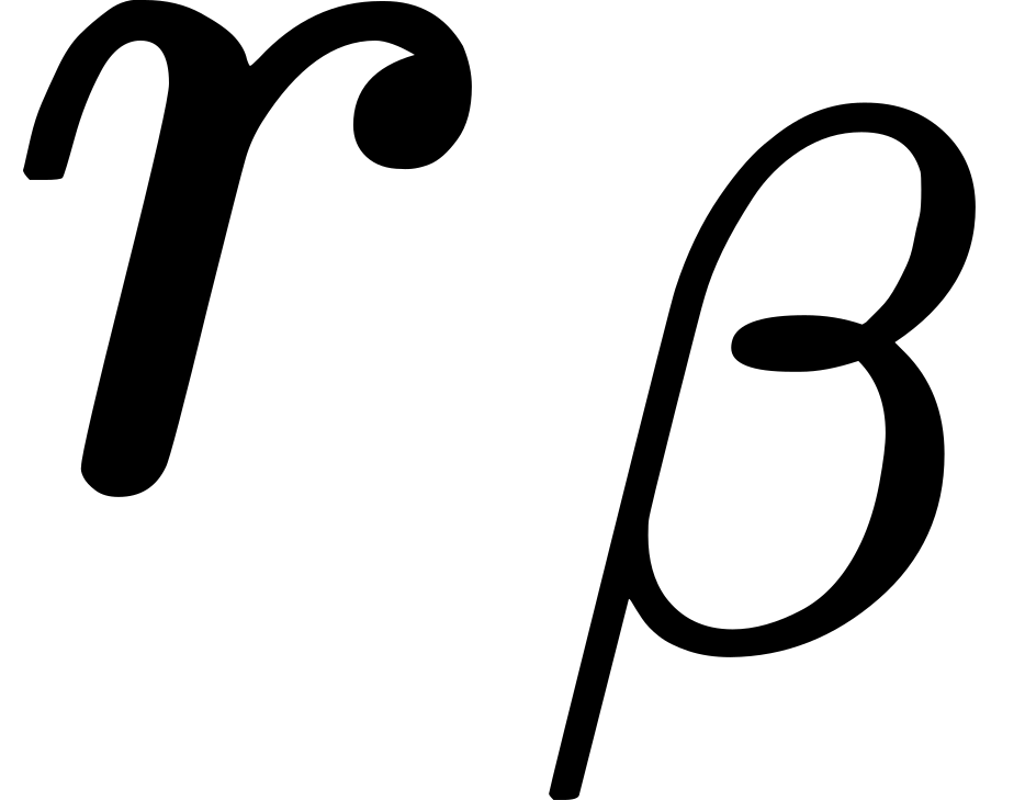 and